QTT on a Physical Interval

The previous tutorial used integer grid indices. This one maps those indices to a real interval, for example [-1, 2]. That is useful when the function is defined as f(x), not as f(i).

Runnable source: docs/tutorial-code/src/bin/qtt_interval.rs

Key API Pieces

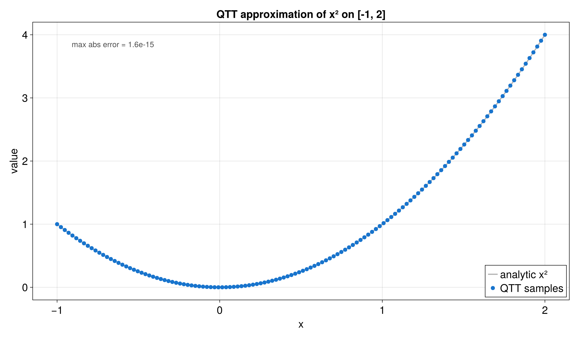
DiscretizedGrid owns the mapping from grid index to physical coordinate. Here the target function is f(x) = x^2 on [-1, 2].

fn main() -> anyhow::Result<()> {
use tensor4all_quanticstci::{
    quanticscrossinterpolate, DiscretizedGrid, QtciOptions, UnfoldingScheme,
};
let grid = DiscretizedGrid::builder(&[7])
    .with_lower_bound(&[-1.0])
    .with_upper_bound(&[2.0])
    .include_endpoint(true)
    .with_unfolding_scheme(UnfoldingScheme::Interleaved)
    .build()?;

let f = |coords: &[f64]| -> f64 {
    let x = coords[0];
    x.powi(2)
};
let options = QtciOptions::default()
    .with_verbosity(0);
let (qtt, _ranks, _errors) = quanticscrossinterpolate(&grid, f, None, options)?;

assert!((qtt.evaluate(&[128])? - 4.0).abs() < 1e-8);
Ok(())
}

Indices passed to evaluate are one-based grid indices. The grid converts them to the physical coordinate before the function is sampled. Passing None for the optional initial-pivot argument keeps the tutorial on the default QTCI initialization path.

What It Computes

The example builds a DiscretizedGrid, evaluates f(x) = x^2 on that grid, and checks that the QTT follows the direct values on the interval.

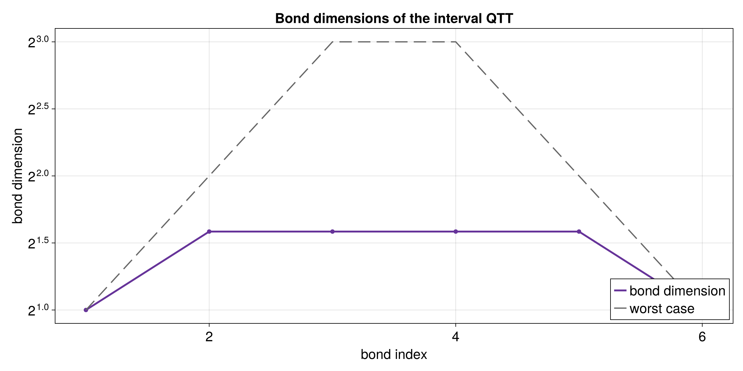
The bond-dimension plot shows how much information is carried between QTT sites. For this smooth example, the internal sizes stay modest.