tensor4all-rs

tensor4all-rs is a Rust implementation of tensor network algorithms, focused on:

• Tensor Cross Interpolation (TCI) — adaptive low-rank tensor approximation with TCI2 primary and TCI1 legacy algorithms
• Quantics Tensor Train (QTT) — representation of functions in exponentially fine grids
• Tree Tensor Networks (TreeTN) — tensor networks with arbitrary tree topology

The library is structured as a workspace of independent crates under crates/, designed for modular use and AI-agentic development workflows. Language bindings for Julia are provided through the C API layer.

Source code and issue tracker: github.com/tensor4all/tensor4all-rs

The repository root README.md stays intentionally concise. Longer runnable examples live in this guide and the guide examples are exercised in CI.

Where to start

Feature highlights

• Dynamic Index/Tensor system inspired by ITensors.jl: indices carry semantic identity, tensor contraction aligns axes by index rather than position
• Tensor Cross Interpolation (TCI): approximates high-dimensional tensors from a small number of evaluations using cross-approximation; TCI2 is the primary algorithm and TCI1 is available for legacy parity
• Quantics Tensor Train (QTT): represents smooth functions on exponentially fine grids; includes transformation operators (affine, shift, sum)
• Tree Tensor Networks: arbitrary-topology TTN, not limited to chains (MPS/MPO); supports standard MPS/MPO as special cases with runtime topology checks
• C API (tensor4all-capi): FFI surface for language bindings, currently used by Tensor4all.jl. This repository is early development with no backward-compatibility guarantee; the C ABI should not be treated as stable.

Not sure where you fit?

If you are new to the library, read Getting Started for a short working example, then consult Concepts for background on the data structures used throughout.

Getting Started

Prerequisites

You need the Rust toolchain. If you do not have it installed, follow the instructions at https://rustup.rs/.

Adding tensor4all-rs to Your Project

tensor4all-rs is a collection of crates. The crates are not published to crates.io yet, so use git dependencies from an external project:

[dependencies]
# Basic tensor train construction and manipulation
tensor4all-simplett = { git = "https://github.com/tensor4all/tensor4all-rs", package = "tensor4all-simplett" }

# Indexed tensors and ITensors-like TensorTrain/TT-SVD
tensor4all-core = { git = "https://github.com/tensor4all/tensor4all-rs", package = "tensor4all-core" }
tensor4all-itensorlike = { git = "https://github.com/tensor4all/tensor4all-rs", package = "tensor4all-itensorlike" }

# Tensor Cross Interpolation (TCI)
tensor4all-tensorci = { git = "https://github.com/tensor4all/tensor4all-rs", package = "tensor4all-tensorci" }

# Quantics TCI (combines quantics encoding with TCI)
tensor4all-quanticstci = { git = "https://github.com/tensor4all/tensor4all-rs", package = "tensor4all-quanticstci" }

# Tree tensor networks
tensor4all-treetn = { git = "https://github.com/tensor4all/tensor4all-rs", package = "tensor4all-treetn" }

You do not need to add all of them — only include the crates relevant to your use case.

When working from a local checkout, use path dependencies instead. Paths are relative to your project’s Cargo.toml; adjust ../tensor4all-rs as needed:

[dependencies]
tensor4all-simplett = { path = "../tensor4all-rs/crates/tensor4all-simplett" }
tensor4all-core = { path = "../tensor4all-rs/crates/tensor4all-core" }
tensor4all-itensorlike = { path = "../tensor4all-rs/crates/tensor4all-itensorlike" }
tensor4all-tensorci = { path = "../tensor4all-rs/crates/tensor4all-tensorci" }
tensor4all-quanticstci = { path = "../tensor4all-rs/crates/tensor4all-quanticstci" }
tensor4all-treetn = { path = "../tensor4all-rs/crates/tensor4all-treetn" }

First Example: Tensor Trains

The following example uses tensor4all-simplett to create a constant tensor train, evaluate it at a specific index, and compress it.

use tensor4all_simplett::prelude::*;

fn main() {
    // Create a constant tensor train with local dimensions [2, 3, 4].
    // Every entry of the represented tensor equals 1.0.
    let tt = SimpleTensorTrain::<f64>::constant(&[2, 3, 4], 1.0);

    // Evaluate at a specific multi-index.
    let value = tt.evaluate(&[0, 1, 2]).unwrap();
    assert!((value - 1.0).abs() < 1e-12);

    // Sum over all indices (2 * 3 * 4 = 24 elements, all 1.0).
    let total = tt.sum();
    assert!((total - 24.0).abs() < 1e-12);

    // Compress with a truncation tolerance.
    let options = CompressionOptions {
        tolerance: 1e-10,
        max_bond_dim: Some(20),
        ..Default::default()
    };
    let compressed = tt.compressed(&options).unwrap();
    assert!((compressed.sum() - 24.0).abs() < 1e-10);

    println!("sum = {}", compressed.sum());
}

Run it with:

cargo run

Next Steps

• Concepts — learn about tensor trains, bond dimensions, and TCI before diving deeper.
• Dense Tensor to Tensor Train with TT-SVD — decompose an existing full indexed tensor with sequential SVD.
• Guides — step-by-step walkthroughs for tensor basics, TCI, quantics transforms, and tree tensor networks.

Concepts

This page introduces the core ideas behind tensor4all-rs in plain language. No deep mathematical background is assumed.

Tensor Train (TT / MPS)

A tensor train (TT) represents a high-dimensional tensor as a chain of smaller, 3-index tensors. Instead of storing all entries of a size-d^N tensor (which grows exponentially with N), a TT stores N tensors each of modest size, multiplied together to reproduce any entry on demand. The size of the shared “bond” indices between adjacent tensors is called the bond dimension m; larger m means a more accurate approximation at the cost of more memory and compute. In quantum physics the same structure is called a Matrix Product State (MPS).

A[0] ---- A[1] ---- A[2] ---- ... ---- A[N-1]
  |          |          |                  |
 i_0        i_1        i_2             i_{N-1}

Vertical lines are site indices (also called physical indices) — one per tensor, labeling the dimension of the original tensor at that position. Horizontal lines are link indices (bond indices) — internal indices that connect neighboring tensors and whose size is the bond dimension.

Tensor Cross Interpolation (TCI)

Tensor Cross Interpolation approximates a high-dimensional function f(i_0, i_1, ..., i_{N-1}) by evaluating it at an adaptively chosen subset of points and fitting a tensor train. The idea generalises the CUR matrix decomposition — which approximates a matrix using selected rows and columns — to arbitrary numbers of dimensions. The algorithm automatically identifies the most informative “pivots” (evaluation points), so it never needs to query the function at every grid point. For smooth or structured functions, the number of required evaluations can be orders of magnitude smaller than the full grid. The output is a tensor train whose accuracy is controlled by a relative tolerance threshold (rtol).

Quantics Tensor Train (QTT)

Quantics (also called quantized tensor train) is a technique for representing functions of continuous variables with a tensor train. A function f(x) sampled on a uniform grid of 2^R points in [0, 1) is reshaped into an R-site tensor train where every site index has dimension 2. Each site corresponds to one bit of the binary representation of the grid index. Smooth functions have low bond dimension in this representation, giving exponential compression relative to storing all 2^R values. Combining QTT with TCI (“Quantics TCI”) allows efficient approximation of high-dimensional continuous integrands without ever forming the full grid.

bit R-1        bit R-2                bit 0
  |              |          ...          |
 B[0] --------- B[1] ----- ... ------- B[R-1]

Each tensor B[k] has two physical legs of dimension 2 (one per variable dimension in the multivariate case) and one or two bond legs.

Tree Tensor Network (TreeTN)

A Tree Tensor Network generalises the tensor train to tree-shaped graphs. Each node of the tree holds a tensor, and each edge corresponds to a shared (bond) index between the two tensors at its endpoints. Contracting along any edge multiplies those two tensors and merges their free indices. The tensor train is the special case where the tree is a simple path graph. Tree structures can capture correlations that are not naturally captured by a chain, making them useful for problems with hierarchical or multi-scale structure. In tensor4all-rs, TreeTensorNetwork<V> (where V is a vertex label type) is the primary data structure representing both TT/MPS and more general tree networks.

         T[root]
        /        \
    T[a]          T[b]
    /   \            \
T[c]   T[d]         T[e]
  |      |             |
 i_c    i_d           i_e

Vertical lines are site indices; lines along the tree edges are bond indices.

Key Terminology

Architecture & Crate Guide

This page describes how tensor4all-rs is organised, what each crate does, how to choose the right crate for your use case, and the two-stack design that keeps the public API predictable.

Two stacks, no facade

The workspace is organised as two independent stacks. Each stack owns its tensor-train representation and its algorithm crates. There is no facade crate that wraps everything: tensor4all-capi is a C FFI layer, not a Rust facade, and each crate can be used on its own.

                        tensor4all-core (Index, Tensor, contraction, SVD/QR)
                                      |
              +-----------------------+------------------------+
              |                                                |
   NETWORK STACK (tree-based)                     SIMPLETT STACK (positional)
              |                                                |
   tensor4all-treetn  (TreeTN)                    tensor4all-simplett (SimpleTensorTrain)
              |                                                |
   tensor4all-itensorlike (TensorTrain)           tensor4all-tensorci (TCI1/TCI2)
              |                                                |
   tensor4all-partitionedtreetn (TreeTN patches)    tensor4all-quanticstci
              |                                                |
   tensor4all-partitionedtt (deprecated)            tensor4all-quanticstransform
              |
   tensor4all-treetci

   tensor4all-capi  (C FFI for language bindings; depends on both stacks)
   tensor4all-hdf5  (MPS serialization, ITensors.jl-compatible)

The sanctioned crossing: treetn::simplett_bridge

The only sanctioned place where the two stacks convert into each other is treetn::simplett_bridge:

• tensor_train_to_treetn / tensor_train_to_treetn_with_names / tensor_train_to_treetn_with_names_and_site_indices: simplett SimpleTensorTrain -> network TreeTN;
• treetn_to_tensor_train: network TreeTN (linear chain) -> simplett SimpleTensorTrain;
• fix_and_remove_site_from_treetn_chain, insert_onehot_site_in_treetn_chain, weighted_remove_site_from_treetn_chain: chain-topology helpers.

Crates that need to cross stacks must route through this bridge. New ad hoc bridges (hand-rolled conversion logic inside another crate) are rejected. tensor4all-partitionedtt consumes simplett output (TCI2 results) only via tensor_train_to_treetn; the TreeTN-native tensor4all-partitionedtreetn operates directly on named TreeTN<IdxTensor, V> values and does not depend on simplett, itensorlike, or TCI crates.

One deliberate exception exists: tensor4all-quanticstransform builds TreeTN-based LinearOperators from simplett MPO data (two site indices per node) via tensortrain_to_linear_operator. That is operator construction, not a general stack conversion: the bridge stays MPS-shaped (one site index per node), and the transform layer keeps the MPO-specific index bookkeeping. No new ad hoc conversions may be added; MPO conversion belongs in the transform layer, and MPS conversion belongs in the bridge.

Which stack does a new feature crate target?

• Application-level features (operators, evolution, DMRG, TDVP, algorithm composition on a known topology) target the network stack by default (tensor4all-treetn, or tensor4all-itensorlike when ITensors.jl-style semantics are wanted).
• Numerical-core features (cross interpolation, factorizations, quantics kernels) target the simplett stack by default (tensor4all-simplett, tensor4all-tensorci; the former tensor4all-tcicore was dissolved into tensor4all-core, #639).
• A feature that must serve both stacks is implemented in the target stack and exposed through treetn::simplett_bridge; it is not duplicated in both.

Vocabulary conventions

Beyond the naming-policy suffixes (_mut, _into, _batched), the following operation names are unified across crates:

• Inner product: inner_product everywhere. (dot was retired in tensor4all-simplett.)
• Densification: full_tensor materializes a tensor train/MPO into a flat column-major buffer plus shape; to_dense materializes a single tensor into a dense IdxTensor. The distinction is intentional (whole-TT vs one-tensor).
• Canonicalization: treetn uses canonicalize / canonicalize_mut; itensorlike uses orthogonalize (ITensors.jl-compatible vocabulary) for the same center-site normalization. Each stack keeps its standard term; do not introduce a third synonym.
• Options: bond caps use max_bond_dim: Option<usize>; truncation tolerances use SvdTruncationPolicy (rtol/cutoff); sweep counts use nfullsweeps/nsweeps (TreeTN) or nhalfsweeps (itensorlike) as documented in the skills guide.

TensorTrain naming resolution

Two different types are named TensorTrain-family, which is the historical naming trap that PR 3 resolves:

Rules:

• tensor4all-simplett::SimpleTensorTrain is the positional chain type. Prefer it for numerical kernels.
• tensor4all-itensorlike::TensorTrain is the tree-based chain type with named indices, canonical forms, and orthogonality tracking.
• There are no compatibility aliases: TensorTrain alone always means the itensorlike type inside that crate, and simplett code must write SimpleTensorTrain.

The corresponding errors follow the representation names:

They are deliberately separate because combining them would couple the two independent stacks. The distinct names prevent ambiguous imports.

Scalar capability boundaries

Scalar traits are layered capabilities rather than interchangeable numeric aliases:

tensor4all_core::AnyScalar is the only public AnyScalar; it may retain an AD-tracked rank-0 tensor. The internal tensorbackend value is named BackendScalar and is an untracked compact scalar. Do not replace these capability boundaries with one all-purpose supertrait: that would force storage and algorithm requirements onto unrelated generic code.

Layer descriptions

Foundation (internal)

Network stack

Simplett stack

Quantics & transforms

Applications

I/O & bindings

I/O & bindings

Which crate should I use?

Error remedies

Public error types use thiserror, preserve the source error, carry structured fields, and name an actionable remedy in the rustdoc when one is documented. Recurring cases avoid opaque string payloads. cargo clippy is configured with -D clippy::missing_errors_doc -D clippy::missing_panics_doc so every fallible or panicking public function documents its failure modes.

Internal crates

tensor4all-tensorbackend is an implementation detail. The former tensor4all-tcicore crate was dissolved into tensor4all-core (#639): the matrix CI / LUCI / rrLU algorithms, CachedFunction, and MultiIndex now live in core. These are still not part of the application-facing public API surface and their interfaces may change without notice.

Tensor Basics

This guide covers the tensor4all-core crate, which provides the foundation for all tensor operations: indices, tensors, contraction, and factorization.

If you have not set up a dependency yet, add tensor4all-core to your Cargo.toml. Use a git dependency from an external project:

[dependencies]
tensor4all-core = { git = "https://github.com/tensor4all/tensor4all-rs", package = "tensor4all-core" }

Or use a path dependency when working from a local checkout:

[dependencies]
tensor4all-core = { path = "../tensor4all-rs/crates/tensor4all-core" }

Index

Every tensor axis is identified by an Index. Indices carry a unique identity (so two indices with the same dimension are still distinct), an optional tag, and an optional prime level.

#![allow(unused)]
fn main() {
use tensor4all_core::index::{Index, DynId};
use tensor4all_core::IndexLike; // needed for .dim() and .plev()

// Simplest form: just give a dimension.
let i = Index::new_dyn(3);   // dimension 3, auto-generated ID, no tags
let j = Index::new_dyn(4);

// A tag names the index (useful for debugging and tag-based operations).
let site = Index::new_dyn_with_tag(2, "Site").unwrap();
assert_eq!(site.dim(), 2);

// Two indices created independently are always distinct, even with the same dim.
let a = Index::new_dyn(3);
let b = Index::new_dyn(3);
assert_ne!(a, b);

// Prime levels distinguish related indices (e.g. ket vs bra in quantum physics).
let bra = site.prime();       // plev 0 -> 1
let ket = site.noprime();     // always plev 0
assert_ne!(bra, ket);

// Inspect properties.
assert_eq!(site.dim(), 2);
assert_eq!(site.plev(), 0);
assert_eq!(bra.plev(), 1);
}

Tensor (IdxTensor)

IdxTensor is a dynamic-rank tensor parameterized by a list of Index values and backed by compact storage that may be dense, diagonal, or explicitly structured. Each index uniquely identifies an axis; there is no fixed axis ordering in the abstract sense — operations match axes by index identity.

Creating tensors

#![allow(unused)]
fn main() {
use tensor4all_core::{IdxTensor, Index};
use tensor4all_core::index::DynId;

let i = Index::new_dyn(2);
let j = Index::new_dyn(3);

// From explicit column-major data (2×3 tensor, 6 elements).
let data = vec![1.0_f64, 2.0, 3.0, 4.0, 5.0, 6.0];
let t = IdxTensor::from_dense(vec![i.clone(), j.clone()], data).unwrap();
assert_eq!(t.dims(), vec![2, 3]);

// All-zeros tensor.
let zeros = IdxTensor::zeros::<f64>(vec![i.clone(), j.clone()]).unwrap();

// Random tensor (standard normal).
use rand::SeedableRng;
use rand_chacha::ChaCha8Rng;
let mut rng = ChaCha8Rng::seed_from_u64(42);
let rand_t: IdxTensor =
    IdxTensor::random::<f64, _>(&mut rng, vec![i.clone(), j.clone()]).unwrap();
assert_eq!(rand_t.dims(), vec![2, 3]);
}

Extracting data

#![allow(unused)]
fn main() {
use tensor4all_core::{IdxTensor, Index};
use tensor4all_core::index::DynId;

let i = Index::new_dyn(2);
let data = vec![10.0_f64, 20.0];
let t = IdxTensor::from_dense(vec![i], data).unwrap();

// Extract all elements in column-major order.
let out: Vec<f64> = t.to_vec().unwrap();
assert_eq!(out, vec![10.0, 20.0]);

// Sum all elements.
let s = t.sum().unwrap();
assert_eq!(s.real(), 30.0);
}

Contraction

Contraction sums over all shared (common) indices between two or more tensors. Think of it as a generalization of matrix multiplication.

Pairwise contraction

#![allow(unused)]
fn main() {
use tensor4all_core::{IdxTensor, Index, contract};
use tensor4all_core::index::DynId;

// A[i,j] and B[j,k] — contracting over j gives C[i,k].
let i = Index::new_dyn(2);
let j = Index::new_dyn(3);
let k = Index::new_dyn(4);

let a = IdxTensor::zeros::<f64>(vec![i.clone(), j.clone()]).unwrap();
let b = IdxTensor::zeros::<f64>(vec![j.clone(), k.clone()]).unwrap();

let c = contract(&[&a, &b]).unwrap();
assert_eq!(c.dims(), vec![2, 4]);  // j is summed away
}

Multi-tensor contraction

contract contracts a connected list of tensors. Disconnected inputs are an error; use outer_product explicitly when a tensor product of disconnected pieces is intended.

#![allow(unused)]
fn main() {
use tensor4all_core::{
    IdxTensor, Index, contract, outer_product,
};
use tensor4all_core::index::DynId;

let i = Index::new_dyn(2);
let j = Index::new_dyn(3);
let k = Index::new_dyn(4);
let l = Index::new_dyn(5);

let mut rng = {
    use rand::SeedableRng;
    rand_chacha::ChaCha8Rng::seed_from_u64(0)
};
let a: IdxTensor =
    IdxTensor::random::<f64, _>(&mut rng, vec![i.clone(), j.clone()]).unwrap();
let b: IdxTensor =
    IdxTensor::random::<f64, _>(&mut rng, vec![j.clone(), k.clone()]).unwrap();
let c: IdxTensor =
    IdxTensor::random::<f64, _>(&mut rng, vec![k.clone(), l.clone()]).unwrap();

// Contract A(i,j) * B(j,k) * C(k,l) -> result(i,l)
let result = contract(&[&a, &b, &c]).unwrap();
assert_eq!(result.dims().iter().product::<usize>(), 2 * 5); // i * l

// Disconnected products are explicit.
let product = outer_product(&a, &c).unwrap();
assert_eq!(product.dims().iter().product::<usize>(), 2 * 3 * 4 * 5);
}

Factorization

The unified factorize() function dispatches to SVD, QR, LU, or CI based on FactorizeOptions. The result splits the input tensor into a left and right factor connected by a new bond index.

SVD with truncation

#![allow(unused)]
fn main() {
use tensor4all_core::{IdxTensor, Index, factorize, FactorizeOptions, SvdTruncationPolicy};
use tensor4all_core::index::DynId;

let i = Index::new_dyn(4);
let j = Index::new_dyn(6);

let mut rng = {
    use rand::SeedableRng;
    rand_chacha::ChaCha8Rng::seed_from_u64(1)
};
let t: IdxTensor =
    IdxTensor::random::<f64, _>(&mut rng, vec![i.clone(), j.clone()]).unwrap();

// SVD: split along i | j, discarding singular values below the chosen policy threshold.
let opts = FactorizeOptions::svd().with_svd_policy(SvdTruncationPolicy::new(1e-10));
let result = factorize(&t, &[i.clone()], &opts).unwrap();

// result.left  has indices [i, bond]
// result.right has indices [bond, j]
// result.left * result.right ≈ t  (within tolerance)
let bond_dim = result.rank;
println!("bond dimension after SVD: {bond_dim}");

// Limit bond dimension explicitly.
let opts_capped = FactorizeOptions::svd().with_max_bond_dim(2);
let result_capped = factorize(&t, &[i], &opts_capped).unwrap();
assert!(result_capped.rank <= 2);
}

QR decomposition

#![allow(unused)]
fn main() {
use tensor4all_core::{IdxTensor, Index, factorize, FactorizeOptions};
use tensor4all_core::index::DynId;

let i = Index::new_dyn(4);
let j = Index::new_dyn(6);

let mut rng = {
    use rand::SeedableRng;
    rand_chacha::ChaCha8Rng::seed_from_u64(2)
};
let t: IdxTensor =
    IdxTensor::random::<f64, _>(&mut rng, vec![i.clone(), j.clone()]).unwrap();

// QR: left factor is orthogonal (Q), right factor is upper-triangular (R).
let opts = FactorizeOptions::qr();
let result = factorize(&t, &[i], &opts).unwrap();
// result.left  = Q  (orthogonal columns)
// result.right = R  (upper triangular)
}

Both FactorizeOptions::svd() and FactorizeOptions::qr() return builder structs. Use .with_svd_policy(policy) for SVD and .with_qr_rtol(tol) for QR-specific rank control. with_max_bond_dim(n) remains available as an algorithm-independent hard cap. For SVD, result.singular_values holds the retained singular values.

Tensor Train

A Tensor Train (TT), also known as a Matrix Product State (MPS), represents a high-dimensional tensor as a chain of low-rank cores. tensor4all-rs provides two complementary implementations:

When to choose which: Use tensor4all-simplett when you want fast numerics with minimal boilerplate (no named indices needed). Use tensor4all-itensorlike when you need named indices, automatic orthogonality tracking, or ITensors.jl compatibility. If you already have a full IdxTensor, follow Dense Tensor to Tensor Train with TT-SVD.

SimpleTT

The tensor4all-simplett crate offers a minimal, efficient TT implementation. It works with plain f64 and Complex64 scalars and does not require you to manage named indices.

Creating a tensor train

fn main() -> anyhow::Result<()> {
use tensor4all_simplett::prelude::*;

// Constant TT: all entries equal to 1.0, physical dimensions [2, 3, 4]
let tt = SimpleTensorTrain::<f64>::constant(&[2, 3, 4], 1.0);
assert_eq!(tt.len(), 3);
assert_eq!(tt.site_dims(), vec![2, 3, 4]);
assert_eq!(tt.link_dims(), vec![1, 1]); // bond dim = 1 for a constant

// Zero TT: all entries are zero
let zero_tt = SimpleTensorTrain::<f64>::zeros(&[2, 3, 4]);
assert!((zero_tt.sum()).abs() < 1e-14);
Ok(())
}

Evaluating and summing

fn main() -> anyhow::Result<()> {
use tensor4all_simplett::prelude::*;
let tt = SimpleTensorTrain::<f64>::constant(&[2, 3, 4], 1.0);
// Evaluate the tensor at a specific multi-index
let value = tt.evaluate(&[0, 1, 2])?;
assert!((value - 1.0).abs() < 1e-12);

// Sum over all multi-indices (equivalent to contracting with all-ones vectors)
let total = tt.sum();
// For the constant TT: sum = 1.0 * 2 * 3 * 4 = 24.0
assert!((total - 24.0).abs() < 1e-10);
Ok(())
}

Compressing

CompressionOptions controls the accuracy–cost trade-off:

fn main() -> anyhow::Result<()> {
use tensor4all_simplett::prelude::*;
// Build a TT with artificially inflated bond dimension by adding two constants
let a = SimpleTensorTrain::<f64>::constant(&[2, 3, 4], 1.0);
let b = SimpleTensorTrain::<f64>::constant(&[2, 3, 4], 2.0);
let big = a.add(&b)?; // bond dim = 2, but rank-1 would suffice
assert_eq!(big.rank(), 2);

let options = CompressionOptions {
    tolerance: 1e-10,
    max_bond_dim: Some(20),
    ..Default::default()
};
let compressed = big.compressed(&options)?;

// Compression found the optimal rank
assert_eq!(compressed.rank(), 1);
// Values are preserved: 1.0 + 2.0 = 3.0
assert!((compressed.evaluate(&[0, 1, 2])? - 3.0).abs() < 1e-10);
Ok(())
}

The compression reduces bond dimensions while keeping the approximation error below tolerance (relative truncation threshold), up to max_bond_dim.

Tolerance guidance:

• 1e-12 (default): near machine precision, almost lossless.
• 1e-8 to 1e-6: good for most scientific applications.
• Tighter tolerances produce larger bond dimensions and slower evaluation.

End-to-end workflow

This example shows the complete lifecycle: create, add, compress, evaluate, and verify.

fn main() -> anyhow::Result<()> {
use tensor4all_simplett::prelude::*;

// Step 1: Create two constant TTs
let a = SimpleTensorTrain::<f64>::constant(&[4, 4, 4], 1.0);
let b = SimpleTensorTrain::<f64>::constant(&[4, 4, 4], 2.0);

// Step 2: Add them (bond dim doubles)
let sum = a.add(&b)?;
assert_eq!(sum.rank(), 2);

// Step 3: Compress
let compressed = sum.compressed(&CompressionOptions::default())?;
assert_eq!(compressed.rank(), 1);

// Step 4: Evaluate and verify
for i in 0..4 {
    for j in 0..4 {
        let val = compressed.evaluate(&[i, j, 0])?;
        assert!((val - 3.0).abs() < 1e-10);
    }
}

// Step 5: Check norm
// norm^2 = 3^2 * 4^3 = 576, norm = 24
assert!((compressed.norm() - 24.0).abs() < 1e-10);
Ok(())
}

ITensorLike TensorTrain

The tensor4all-itensorlike crate provides a higher-level API modelled after ITensorMPS.jl. Each tensor carries named DynIndex objects so that contractions are unambiguous regardless of axis ordering.

Key conventions

• Sites are 0-indexed (Julia uses 1-indexed).
• IdxTensor::from_dense expects data in column-major (Fortran) order.
• inner() computes <self|other> with complex conjugation on self.

Creating and orthogonalizing

fn main() -> anyhow::Result<()> {
use tensor4all_itensorlike::prelude::*;

// Site and bond indices
let s0 = DynIndex::new_dyn(2);
let s1 = DynIndex::new_dyn(2);
let s2 = DynIndex::new_dyn(2);
let b01 = DynIndex::new_bond(2)?;
let b12 = DynIndex::new_bond(2)?;

// Build site tensors (column-major data)
let t0 = IdxTensor::from_dense(
    vec![s0.clone(), b01.clone()],
    vec![1.0_f64, 0.0, 0.0, 1.0],
)?;
let t1 = IdxTensor::from_dense(
    vec![b01.clone(), s1.clone(), b12.clone()],
    vec![1.0, 0.0, 0.0, 1.0, 0.0, 1.0, 1.0, 0.0],
)?;
let t2 = IdxTensor::from_dense(
    vec![b12.clone(), s2.clone()],
    vec![1.0, 0.0, 0.0, 1.0],
)?;

// Assemble and orthogonalize with center at site 1
let mut tt = TensorTrain::new(vec![t0, t1, t2])?;
let norm_before = tt.norm()?;
tt.orthogonalize(1)?;

assert!(tt.is_ortho());
assert_eq!(tt.ortho_center(), Some(1));

// Orthogonalization preserves the tensor train value
assert!((tt.norm()? - norm_before).abs() < 1e-10);
Ok(())
}

Truncating

After orthogonalization you can truncate bond dimensions by SVD:

fn main() -> anyhow::Result<()> {
use tensor4all_itensorlike::prelude::*;
let s0 = DynIndex::new_dyn(2);
let s1 = DynIndex::new_dyn(2);
let s2 = DynIndex::new_dyn(2);
let b01 = DynIndex::new_bond(4)?;
let b12 = DynIndex::new_bond(4)?;
let t0 = IdxTensor::from_dense(
    vec![s0, b01.clone()],
    (0..8).map(|i| i as f64).collect(),
)?;
let t1 = IdxTensor::from_dense(
    vec![b01, s1, b12.clone()],
    (0..32).map(|i| i as f64).collect(),
)?;
let t2 = IdxTensor::from_dense(
    vec![b12, s2],
    (0..8).map(|i| i as f64).collect(),
)?;
let mut tt = TensorTrain::new(vec![t0, t1, t2])?;
tt.orthogonalize(1)?;
tt.truncate(
    &TruncateOptions::svd()
        .with_svd_policy(tensor4all_core::SvdTruncationPolicy::new(1e-10))
        .with_max_bond_dim(2),
)?;
assert!(tt.max_bond_dim() <= 2);
Ok(())
}

SvdTruncationPolicy::new(threshold) uses the default relative per-value rule. To emulate ITensor-style discarded-weight cutoffs, use .with_squared_values().with_discarded_tail_sum().

Norm and inner product

fn main() -> anyhow::Result<()> {
use tensor4all_itensorlike::prelude::*;
let s0 = DynIndex::new_dyn(2);
let s1 = DynIndex::new_dyn(2);
let b = DynIndex::new_bond(2)?;
let t0 = IdxTensor::from_dense(
    vec![s0, b.clone()],
    vec![1.0_f64, 0.0, 0.0, 1.0],
)?;
let t1 = IdxTensor::from_dense(
    vec![b, s1],
    vec![1.0, 0.0, 0.0, 1.0],
)?;
let tt = TensorTrain::new(vec![t0, t1])?;
let norm = tt.norm()?;
assert!(norm.is_finite());

// <tt|tt> = ||tt||^2
let inner = tt.inner(&tt)?;
assert!((inner.real() - norm * norm).abs() < 1e-10);
Ok(())
}

Complex scalars

The same API works with Complex64:

fn main() -> anyhow::Result<()> {
use num_complex::Complex64;
use tensor4all_itensorlike::prelude::*;

let s0 = DynIndex::new_dyn(2);
let s1 = DynIndex::new_dyn(2);
let b  = DynIndex::new_bond(2)?;

let t0 = IdxTensor::from_dense(
    vec![s0, b.clone()],
    vec![
        Complex64::new(1.0,  0.0), Complex64::new(0.0,  1.0),
        Complex64::new(0.0, -1.0), Complex64::new(1.0,  0.0),
    ],
)?;
let t1 = IdxTensor::from_dense(
    vec![b, s1],
    vec![
        Complex64::new(1.0, 0.0), Complex64::new(0.0, 0.0),
        Complex64::new(0.0, 0.0), Complex64::new(1.0, 0.0),
    ],
)?;

let tt = TensorTrain::new(vec![t0, t1])?;

// Norm is sqrt(<tt|tt>) = sqrt(conj(tt) * tt summed over all indices)
let norm = tt.norm()?;
assert!(norm > 0.0);

// For complex tensors, inner product uses complex conjugation on self
let inner = tt.inner(&tt)?;
assert!((inner.real() - norm * norm).abs() < 1e-10);
Ok(())
}

Differences from ITensorMPS.jl

Dense Tensor to Tensor Train with TT-SVD

Use TensorTrain::from_dense when all values of an indexed tensor already fit in memory and you want a sequential SVD decomposition. For sampled functions whose full tensor does not fit in memory, use TCI instead.

Complete example

fn main() -> anyhow::Result<()> {
use tensor4all_core::{DynIndex, IdxTensor, SvdTruncationPolicy};
use tensor4all_itensorlike::{CanonicalForm, SvdOptions, TensorTrain};
let sites = [
    DynIndex::new_dyn(2),
    DynIndex::new_dyn(2),
    DynIndex::new_dyn(2),
];

// IdxTensor dense buffers are column-major: sites[0] varies fastest.
// These values are [1, 2] ⊗ [1, 3] ⊗ [1, 4].
let dense = IdxTensor::from_dense(
    sites.to_vec(),
    vec![1.0, 2.0, 3.0, 6.0, 4.0, 8.0, 12.0, 24.0],
)?;
let options = SvdOptions::new()
    .with_policy(SvdTruncationPolicy::new(1.0e-12))
    .with_max_bond_dim(16);
let train = TensorTrain::from_dense(&dense, &sites, &options)?;

let reconstructed = train.to_dense()?;
assert!(dense.distance(&reconstructed)? < 1.0e-12);
assert_eq!(train.bond_dims(), vec![1, 1]);
assert_eq!(train.ortho_center(), Some(2));
assert_eq!(train.canonical_form(), Some(CanonicalForm::Unitary));
Ok(())
}

The sites slice defines the tensor-train order. It must contain every full DynIndex of the input exactly once, but it need not match the input tensor’s axis order. Prime levels and tags are part of index identity.

Sweep and canonical form

TT-SVD splits from left to right. At each bond, U becomes the completed left-canonical core and S Vᴴ is carried into the next split. The final core therefore holds the remaining norm, and the returned train records the final site as its orthogonality center.

Truncation

SvdOptions has two independent controls:

• with_policy(...) chooses which singular-value tail is discarded at each bond;
• with_max_bond_dim(n) caps every retained bond at n.

For a discarded-Frobenius-weight rule, use squared singular values and a tail sum:

#![allow(unused)]
fn main() {
use tensor4all_core::SvdTruncationPolicy;
let local_policy = SvdTruncationPolicy::new(1.0e-10)
    .with_squared_values()
    .with_discarded_tail_sum();
assert_eq!(local_policy.threshold, 1.0e-10);
}

The policy is applied separately at each of the number_of_sites - 1 splits. It is therefore not, by itself, a statement of the final global relative error. When a global tolerance matters, allocate a tighter per-bond error budget and verify the result with dense.distance(&train.to_dense()?), as in the example. A hard max_bond_dim can force a larger error regardless of the policy.

Memory cost

This is an explicitly dense algorithm. The input already costs the product of all site dimensions, and SVD workspaces plus the carried tensor can require several times that storage. Do not use dense TT-SVD as a hidden compression path for data that cannot already be materialized. Use TCI for oracle-defined or otherwise non-materialized data.

Tensor Cross Interpolation

Tensor Cross Interpolation (TCI) approximates a high-dimensional function as a tensor train by sampling only a small fraction of its entries. This crate provides two levels of API:

• tensor4all-tensorci for low-level TCI directly on integer indices.
• tensor4all-quanticstci for quantics interpolation on discrete or continuous grids.

Low-Level TCI (tensor4all-tensorci)

Use crossinterpolate2 when you already know the local dimensions and want direct control over the algorithm.

Defining the function

The function must accept a &Vec<usize> of 0-indexed multi-indices and return a scalar value. Here is a simple 2D example where f(i, j) = i + j + 1:

#![allow(unused)]
fn main() {
use tensor4all_simplett::prelude::*;
use tensor4all_tensorci::prelude::*;

let f = |idx: &Vec<usize>| (idx[0] + idx[1] + 1) as f64;
let local_dims = vec![4, 4];
let initial_pivots = vec![vec![3, 3]]; // pick where |f| is large

let result = crossinterpolate2::<f64, _, fn(&[Vec<usize>]) -> Vec<f64>>(
    f,
    None,
    local_dims,
    initial_pivots,
    TCI2Options {
        tolerance: 1e-10,
        seed: Some(42),
        ..Default::default()
    },
).unwrap();

assert_eq!(result.termination, TCI2Termination::Converged);

let tt = result.tci.to_tensor_train().unwrap();
let value = tt.evaluate(&[2, 3]).unwrap();
assert!((value - 6.0).abs() < 1e-10);
assert!(tt.rank() >= 1);
}

Choosing TCI2Options

The most important parameters:

Interpreting the results

crossinterpolate2 returns a TCI2OptimizationResult:

Do not infer convergence from errors.last() alone. Full convergence also requires no recent global pivots and a stable rank history.

Convergence diagnostics

The errors vector tracks the normalized bond error after each half-sweep. The algorithm converges when:

1. The last ncheck_history (default: 3) entries are all below tolerance.
2. No global pivots were added in those iterations.
3. The rank has stabilized.

If the errors plateau above your tolerance, try:

• Increasing max_bond_dim (the function may need higher rank).
• Increasing max_iter (more sweeps may be needed).
• Choosing better initial pivots (where |f| is large).

Convert to a tensor train for further manipulation:

#![allow(unused)]
fn main() {
use tensor4all_simplett::prelude::*;
use tensor4all_tensorci::prelude::*;
let f = |idx: &Vec<usize>| (idx[0] + idx[1] + 1) as f64;
let tensor4all_tensorci::TCI2OptimizationResult { tci, ranks: _ranks, errors: _errors, .. } = crossinterpolate2::<f64, _, fn(&[Vec<usize>]) -> Vec<f64>>(
    f, None, vec![4, 4], vec![vec![3, 3]],
    TCI2Options { seed: Some(42), ..Default::default() },
).unwrap();
let tt = tci.to_tensor_train().unwrap();
assert!(tt.rank() >= 1);

// Evaluate the tensor train at specific indices
let val = tt.evaluate(&[1, 2]).unwrap();
assert!((val - 4.0).abs() < 1e-10); // f(1,2) = 1+2+1 = 4
}

Continuous vs discrete

crossinterpolate2 works on discrete integer indices. For functions on continuous domains, use the quantics representation provided by tensor4all-quanticstci (see below), which maps floating-point coordinates to binary tensor-train indices.

High-Level Quantics TCI (tensor4all-quanticstci)

The quantics representation encodes each grid index in binary and arranges the bits across tensor-train sites. This often yields much lower bond dimensions than a naive encoding.

Important conventions

• Indexing differs between the two APIs:
  • crossinterpolate2 (low-level): indices and pivots are 0-indexed (0..local_dim)
  • quanticscrossinterpolate_discrete (high-level): grid indices are 0-indexed (0..grid_size)
• Equal dimensions: quanticscrossinterpolate_discrete requires all dimensions to have the same number of points.
• Power-of-2 grid sizes: all grid dimensions must be powers of 2 (4, 8, 16, 32, …).

Choosing between discrete and continuous APIs

Tip on n_random_init_pivot: The n_random_init_pivot option (default: 5) controls how many random initial pivot points are used to seed the TCI algorithm. For functions with multiple separated features or high-dimensional problems, increase this to 10–20 to improve robustness.

Discrete grid interpolation

Use quanticscrossinterpolate_discrete when your function is naturally defined on an integer grid. Indices are passed as &[usize] and are 0-indexed.

fn main() -> anyhow::Result<()> {
use tensor4all_quanticstci::prelude::*;

let f = |idx: &[usize]| (idx[0] + idx[1]) as f64;
let sizes = vec![16, 16];

let (qtci, ranks, errors) = quanticscrossinterpolate_discrete::<f64, _>(
    &sizes,
    f,
    None,
    QtciOptions::default().with_tolerance(1e-10),
)?;

assert!(*errors.last().unwrap() < 1e-10);
assert!(!ranks.is_empty());

let value = qtci.evaluate(&[5, 10])?;
assert!((value - 15.0).abs() < 1e-8);

// Sum of (i + j) for i, j in 0..16 = 2 * 16 * (15 * 16 / 2) = 3840
let total = qtci.sum()?;
assert!((total - 3840.0).abs() < 1e-6);
Ok(())
}

Continuous grid interpolation with DiscretizedGrid

For functions on continuous domains, build a DiscretizedGrid that maps grid indices to physical coordinates. The number of quantics bits per dimension is set via the builder.

fn main() -> anyhow::Result<()> {
use tensor4all_quanticstci::prelude::*;

// 2^4 = 16 grid points on [0, 1)
let grid = DiscretizedGrid::builder(&[4])
    .with_lower_bound(&[0.0])
    .with_upper_bound(&[1.0])
    .build()
    .unwrap();

let f = |x: &[f64]| x[0] * x[0];

let (qtci, _ranks, errors) = quanticscrossinterpolate::<f64, _>(
    &grid,
    f,
    None,
    QtciOptions::default(),
)?;

assert!(*errors.last().unwrap() < 1e-8);

// Verify the interpolation at grid point 0 (x = 0.0)
let value = qtci.evaluate(&[0])?;
assert!((value - 0.0).abs() < 1e-10);
Ok(())
}

Integration

integral() computes a left Riemann sum:

integral ≈ Σ f(xᵢ) × Δx

This has O(h) convergence where h is the grid spacing. The result depends on whether include_endpoint is set on the DiscretizedGrid.

fn main() -> anyhow::Result<()> {
use tensor4all_quanticstci::prelude::*;
let grid = DiscretizedGrid::builder(&[4])
    .with_lower_bound(&[0.0])
    .with_upper_bound(&[1.0])
    .build()
    .unwrap();
let f = |x: &[f64]| x[0] * x[0];
let (qtci, _, _) = quanticscrossinterpolate::<f64, _>(
    &grid, f, None, QtciOptions::default(),
)?;
let integral = qtci.integral()?;
// Left Riemann sum of x^2 over [0, 1) with 16 points
assert!((integral - 1.0 / 3.0).abs() < 5e-2);

let sum = qtci.sum()?;
assert!((sum * grid.grid_step()[0] - integral).abs() < 1e-12);
Ok(())
}

For discrete grids created without a continuous domain, integral() returns the plain sum identical to sum().

Practical Example: Multi-scale 1D Function

This section corresponds to the Julia Quantics TCI of univariate function notebook.

The function below mixes several length scales:

f(x) = cos(x/B) * cos(x/(4*sqrt(5)*B)) * exp(-x^2) + 2*exp(-x)

with B = 2^-30 on [0, ln(20)) using R = 40 quantics bits.

fn main() -> anyhow::Result<()> {
use tensor4all_quanticstci::prelude::*;

// Use R = 10 bits (2^10 = 1024 points) for a fast doctest.
// In practice, set R = 40 for the full multi-scale resolution.
let r = 10;
let x_max = 20.0_f64.ln();
let grid = DiscretizedGrid::builder(&[r])
    .with_lower_bound(&[0.0])
    .with_upper_bound(&[x_max])
    .include_endpoint(false)
    .build()
    .unwrap();

// A smooth multi-scale function: f(x) = cos(10x) * exp(-x^2) + 2*exp(-x)
let f = move |coords: &[f64]| {
    let x = coords[0];
    (10.0 * x).cos() * (-x * x).exp() + 2.0 * (-x).exp()
};

let tol = 1e-8;
let (qtci, _ranks, errors) = quanticscrossinterpolate::<f64, _>(
    &grid,
    f,
    None,
    QtciOptions::default()
        .with_tolerance(tol)
        .with_max_bond_dim(64)
        .with_nrandominitpivot(8),
)?;

assert!(*errors.last().unwrap() < tol);

// Verify at several grid points across the domain
for &grid_idx in &[0usize, 99, 511, 1023] {
    let got = qtci.evaluate(&[grid_idx])?;
    assert!(got.is_finite(), "value at grid index {} should be finite", grid_idx);
}

// Check the integral is reasonable (positive, since f > 0 near x = 0)
let integral = qtci.integral()?;
assert!(integral > 1.0);
Ok(())
}

Multivariate (2D) Example

This section corresponds to the Julia Quantics TCI of multivariate function notebook.

fn main() -> anyhow::Result<()> {
use tensor4all_quanticstci::prelude::*;

// Use 64x64 for a faster doctest (256x256 in practice)
let sizes = vec![64, 64];
let f = |idx: &[usize]| {
    let x = idx[0] as f64;
    let y = idx[1] as f64;
    (x / 24.0).cos() + (y / 17.0).cos() + 0.1 * ((x + y) / 13.0).sin()
};

let (qtci, _ranks, errors) = quanticscrossinterpolate_discrete::<f64, _>(
    &sizes,
    f,
    None,
    QtciOptions::default()
        .with_tolerance(1e-10)
        .with_max_bond_dim(64)
        .with_nrandominitpivot(8),
)?;

assert!(*errors.last().unwrap() < 1e-8);

for &(i, j) in &[(0usize, 0usize), (16, 32), (31, 49), (63, 63)] {
    let exact = (i as f64 / 24.0).cos()
        + (j as f64 / 17.0).cos()
        + 0.1 * (((i + j) as f64) / 13.0).sin();
    let got = qtci.evaluate(&[i, j])?;
    assert!((got - exact).abs() < 1e-6);
}
Ok(())
}

TCI Advanced Topics

This guide corresponds to the Julia Quantics TCI (advanced topics) notebook.

Direct crossinterpolate2 Usage

This path bypasses the high-level quantics wrapper and works directly with quantics bits. Use vec![2; R] as local_dims, because each site is binary.

#![allow(unused)]
fn main() {
use tensor4all_simplett::AbstractTensorTrain;
use tensor4all_tensorci::{crossinterpolate2, TCI2Options, TCI2Termination};

let r = 8;
let local_dims = vec![2; r];
let x_max = 1.0_f64;
let step = x_max / (1usize << r) as f64;

let f = move |idx: &Vec<usize>| {
    let q = idx.iter().fold(0usize, |acc, &bit| (acc << 1) | bit);
    let x = q as f64 * step;
    (-3.0 * x).exp()
};

let initial_pivots = vec![vec![0; r]];
let result = crossinterpolate2::<f64, _, fn(&[Vec<usize>]) -> Vec<f64>>(
    f,
    None,
    local_dims.clone(),
    initial_pivots,
    TCI2Options {
        tolerance: 1e-12,
        seed: Some(42),
        ..Default::default()
    },
).unwrap();

assert_eq!(result.termination, TCI2Termination::Converged);

let tt = result.tci.to_tensor_train().unwrap();
for bits in [
    vec![0, 0, 0, 0, 0, 0, 0, 0],
    vec![1, 0, 0, 0, 0, 0, 0, 0],
    vec![1, 1, 0, 0, 0, 0, 0, 0],
] {
    let q = bits.iter().fold(0usize, |acc, &bit| (acc << 1) | bit);
    let exact = (-3.0 * (q as f64 * step)).exp();
    let got = tt.evaluate(&bits).unwrap();
    assert!((got - exact).abs() < 1e-8);
}
}

Initial Pivot Selection

Choose an initial pivot where |f| is large. That usually helps the first local solve. You can use opt_first_pivot for automatic local search, or pick candidates manually:

#![allow(unused)]
fn main() {
let r = 8;
let x_max = 1.0_f64;
let step = x_max / (1usize << r) as f64;
let f = move |idx: &Vec<usize>| {
    let q = idx.iter().fold(0usize, |acc, &bit| (acc << 1) | bit);
    let x = q as f64 * step;
    (-3.0 * x).exp()
};
let candidates = vec![
    vec![0; r],
    vec![1; r],
    vec![0, 1, 0, 1, 0, 1, 0, 1],
    vec![1, 1, 1, 1, 1, 1, 1, 1],
];

let first_pivot = candidates
    .into_iter()
    .max_by(|a, b| {
        let va = f(a).abs();
        let vb = f(b).abs();
        va.partial_cmp(&vb).unwrap()
    })
    .unwrap();

// f(0,...,0) = exp(0) = 1.0 is the maximum of exp(-3x) on [0,1)
assert_eq!(first_pivot, vec![0; r]);
}

Alternatively, use opt_first_pivot to refine any starting guess:

#![allow(unused)]
fn main() {
use tensor4all_tensorci::opt_first_pivot;

let f = |idx: &Vec<usize>| (idx[0] as f64 + idx[1] as f64 + 1.0).powi(2);
let local_dims = vec![4, 4];
let start = vec![0, 0];

let pivot = opt_first_pivot::<f64, _>(&f, &local_dims, &start, 1000);
assert_eq!(pivot, vec![3, 3]); // f(3,3) = 49.0 is the maximum
}

CachedFunction

Wrap expensive evaluations with CachedFunction to avoid redundant calls. The cache is shared across all TCI sweeps.

#![allow(unused)]
fn main() {
use tensor4all_core::CachedFunction;
use tensor4all_simplett::AbstractTensorTrain;
use tensor4all_tensorci::{crossinterpolate2, TCI2Options};

let r = 8;
let local_dims = vec![2; r];
let x_max = 1.0_f64;
let step = x_max / (1usize << r) as f64;

let cf = CachedFunction::new(
    |idx: &[usize]| {
        let q = idx.iter().fold(0usize, |acc, &bit| (acc << 1) | bit);
        let x = q as f64 * step;
        (-3.0 * x).exp()
    },
    &local_dims,
).unwrap();

let cached_f = |idx: &Vec<usize>| cf.eval(idx).unwrap();
let tensor4all_tensorci::TCI2OptimizationResult { tci: tci_cached, ranks: _ranks, errors: _errors, .. } = crossinterpolate2::<f64, _, fn(&[Vec<usize>]) -> Vec<f64>>(
    cached_f,
    None,
    local_dims.clone(),
    vec![vec![0; r]],
    TCI2Options {
        tolerance: 1e-12,
        seed: Some(42),
        ..Default::default()
    },
).unwrap();

assert!(cf.cache_size() > 0);
assert!(tci_cached.rank() >= 1);

// The cache avoids recomputing values seen in previous sweeps
assert!(cf.num_cache_hits() > 0);
}

Performance guidance

• CachedFunction is most useful when the function evaluation is expensive (e.g., solving a differential equation for each index).
• For cheap functions (arithmetic, elementary functions), the caching overhead may not be worth it.
• The cache grows with the number of unique indices evaluated. For very high-dimensional problems, memory usage may become significant.

Manual Integral

For a uniform half-open grid on [x_min, x_max), the quantics tensor train sum becomes a Riemann integral after multiplying by the cell width:

integral = tt.sum() * (x_max - x_min) / 2^R

#![allow(unused)]
fn main() {
use tensor4all_simplett::AbstractTensorTrain;
use tensor4all_tensorci::{crossinterpolate2, TCI2Options};
let r = 8;
let local_dims = vec![2; r];
let x_max = 1.0_f64;
let step = x_max / (1usize << r) as f64;
let f = move |idx: &Vec<usize>| {
    let q = idx.iter().fold(0usize, |acc, &bit| (acc << 1) | bit);
    let x = q as f64 * step;
    (-3.0 * x).exp()
};
let tensor4all_tensorci::TCI2OptimizationResult { tci, ranks: _ranks, errors: _errors, .. } = crossinterpolate2::<f64, _, fn(&[Vec<usize>]) -> Vec<f64>>(
    f, None, local_dims, vec![vec![0; r]],
    TCI2Options { tolerance: 1e-12, seed: Some(42), ..Default::default() },
).unwrap();
let tt = tci.to_tensor_train().unwrap();
let integral = tt.sum() * (x_max - 0.0) / (1usize << r) as f64;

// For f(x) = exp(-3x) on [0, 1): integral = (1 - e^{-3}) / 3
let exact_integral = (1.0 - (-3.0_f64).exp()) / 3.0;
// R=8 gives 256 grid points; Riemann sum error is O(h) ~ 1/256
assert!((integral - exact_integral).abs() < 1e-2);
}

Compressing Existing Data

This guide corresponds to the Julia Compressing existing data notebook.

Problem

The goal is to compress a large 3D array without materializing the full tensor in memory. Instead of allocating 128 x 128 x 128 values up front, define a function that computes the element on demand and let TCI discover the low-rank structure.

When compression works well: Functions with low-rank structure (sums of separable terms, smooth functions, oscillatory functions). The example below – cos(x) + cos(y) + cos(z) – is a sum of three single-variable functions and has exact TT rank 2.

Tolerance selection: Start with 1e-12 (near machine precision). If the resulting bond dimensions are too large for your application, relax to 1e-8 or 1e-6.

TCI Compression

fn main() -> anyhow::Result<()> {
use std::f64::consts::PI;
use tensor4all_simplett::prelude::*;
use tensor4all_tensorci::prelude::*;

let local_dims = vec![128, 128, 128];
let f = |idx: &Vec<usize>| {
    let x = 2.0 * PI * idx[0] as f64 / 128.0;
    let y = 2.0 * PI * idx[1] as f64 / 128.0;
    let z = 2.0 * PI * idx[2] as f64 / 128.0;
    x.cos() + y.cos() + z.cos()
};

let result = crossinterpolate2::<f64, _, fn(&[Vec<usize>]) -> Vec<f64>>(
    f,
    None,
    local_dims.clone(),
    vec![vec![0, 0, 0]],
    TCI2Options {
        tolerance: 1e-12,
        max_bond_dim: Some(64),
        ..Default::default()
    },
)?;

assert_eq!(result.termination, TCI2Termination::Converged);

let tt = result.tci.to_tensor_train()?;
for point in [
    vec![0, 0, 0],
    vec![1, 2, 3],
    vec![17, 33, 65],
    vec![127, 127, 127],
] {
    let x = 2.0 * PI * point[0] as f64 / 128.0;
    let y = 2.0 * PI * point[1] as f64 / 128.0;
    let z = 2.0 * PI * point[2] as f64 / 128.0;
    let exact = x.cos() + y.cos() + z.cos();
    let got = tt.evaluate(&point)?;
    assert!((got - exact).abs() < 1e-8);
}
Ok(())
}

Compression Quality

The quality of the compression is visible in the bond dimensions and the parameter count of the tensor train.

fn main() -> anyhow::Result<()> {
use std::f64::consts::PI;
use tensor4all_simplett::prelude::*;
use tensor4all_tensorci::prelude::*;
let local_dims = vec![128, 128, 128];
let f = |idx: &Vec<usize>| {
    let x = 2.0 * PI * idx[0] as f64 / 128.0;
    let y = 2.0 * PI * idx[1] as f64 / 128.0;
    let z = 2.0 * PI * idx[2] as f64 / 128.0;
    x.cos() + y.cos() + z.cos()
};
let tensor4all_tensorci::TCI2OptimizationResult { tci, .. } = crossinterpolate2::<f64, _, fn(&[Vec<usize>]) -> Vec<f64>>(
    f, None, local_dims.clone(), vec![vec![0, 0, 0]],
    TCI2Options { tolerance: 1e-12, max_bond_dim: Some(64), ..Default::default() },
)?;
let tt = tci.to_tensor_train()?;
let bond_dims = tt.link_dims();
assert!(!bond_dims.is_empty());

let full_size = local_dims.iter().product::<usize>();
let compressed_params: usize = (0..tt.len())
    .map(|i| {
        let tensor = tt.site_tensor(i);
        tensor.left_dim() * tensor.site_dim() * tensor.right_dim()
    })
    .sum();

let compression_ratio = full_size as f64 / compressed_params as f64;

assert!(compression_ratio > 10.0);
assert!(bond_dims.iter().copied().max().unwrap_or(0) <= 64);
Ok(())
}

Quantics Transform

The tensor4all-quanticstransform crate provides LinearOperator constructors for applying transformations to functions represented as quantics tensor trains. It is a Rust port of the transformation functionality from Quantics.jl.

If you have not set up dependencies yet, add the transform and TreeTN crates to your Cargo.toml. Use git dependencies from an external project:

[dependencies]
tensor4all-quanticstransform = { git = "https://github.com/tensor4all/tensor4all-rs", package = "tensor4all-quanticstransform" }
tensor4all-treetn = { git = "https://github.com/tensor4all/tensor4all-rs", package = "tensor4all-treetn" }

Or use path dependencies when working from a local checkout:

[dependencies]
tensor4all-quanticstransform = { path = "../tensor4all-rs/crates/tensor4all-quanticstransform" }
tensor4all-treetn = { path = "../tensor4all-rs/crates/tensor4all-treetn" }

Operator Overview

Every constructor returns a LinearOperator from tensor4all-treetn, so all operators are applied in the same way regardless of their mathematical meaning.

The parameter r that appears in every constructor is the number of quantics bits (sites) per variable. A single variable is discretized on 2^r grid points.

Error Conditions

Constructors return Err for invalid inputs:

• r == 0 – no sites to operate on
• r == 1 for cumsum_operator, triangle_operator, quantics_fourier_operator – requires at least 2 sites
• r >= 64 for shift_operator – would overflow a 64-bit integer
• NaN or Inf theta for phase_rotation_operator – invalid rotation angle

Creating Operators

#![allow(unused)]
fn main() {
use tensor4all_quanticstransform::{
    flip_operator, shift_operator, phase_rotation_operator,
    cumsum_operator, quantics_fourier_operator,
    BoundaryCondition, FourierOptions,
};

// 8-bit quantics representation (2^8 = 256 grid points)
let r = 8;

// Flip: f(x) = g(2^R - x)
let flip_op = flip_operator(r, BoundaryCondition::Periodic).unwrap();
assert_eq!(flip_op.mpo().node_count(), r);

// Shift by 10: f(x) = g(x + 10) mod 2^R
let shift_op = shift_operator(r, 10, BoundaryCondition::Periodic).unwrap();
assert_eq!(shift_op.mpo().node_count(), r);

// Phase rotation: f(x) = exp(i*pi/4*x) * g(x)
let phase_op = phase_rotation_operator(r, std::f64::consts::PI / 4.0).unwrap();
assert_eq!(phase_op.mpo().node_count(), r);

// Cumulative sum
let cumsum_op = cumsum_operator(r).unwrap();
assert_eq!(cumsum_op.mpo().node_count(), r);

// Fourier transform (forward)
let ft_op = quantics_fourier_operator(r, FourierOptions::forward()).unwrap();
assert_eq!(ft_op.mpo().node_count(), r);
}

Affine Transform

For transformations of the form y = A*x + b with rational coefficients:

#![allow(unused)]
fn main() {
use tensor4all_quanticstransform::{affine_operator, AffineParams, BoundaryCondition};
use num_rational::Rational64;

let r = 4;

// A = [[1, 1], [1, -1]], b = [0, 0]  (2 outputs, 2 inputs)
let a = vec![
    Rational64::from_integer(1), Rational64::from_integer(1),
    Rational64::from_integer(1), Rational64::from_integer(-1),
];
let b = vec![Rational64::from_integer(0), Rational64::from_integer(0)];
let params = AffineParams::new(a, b, 2, 2).unwrap();
let bc = vec![BoundaryCondition::Periodic; 2];
let affine_op = affine_operator(r, &params, &bc).unwrap();
assert_eq!(affine_op.mpo().node_count(), r);
}

Applying Operators to a Tensor Train

Index Mapping Flow

Operators define abstract input and output indices labeled 0, 1, ..., r-1. To apply an operator, bind those abstract indices to the concrete site indices of the target state, then call apply_linear_operator. When the target TreeTN’s quantics sites are tagged as x=1, x=2, …, use apply_linear_operator_to_numbered_tags; otherwise use explicit index binding with apply_linear_operator_to_indices.

Original TreeTN          Operator            Result TreeTN
+----------------+    +----------------+    +----------------+
|  site_idx_0    |--->|  input_0       |    |  output_0      |
|  site_idx_1    |--->|  input_1       |--->|  output_1      |
|  site_idx_2    |--->|  input_2       |    |  output_2      |
|  other_idx     |    |                |    |  other_idx     |  (passes through)
+----------------+    +----------------+    +----------------+

apply_linear_operator:

1. Contracts the operator’s tensors with the TreeTN.
2. Replaces input indices with output indices.
3. Leaves all unrelated indices unchanged.

Apply Method Selection

ApplyOptions controls how the operator-state contraction is performed. Three methods are available, each with different tradeoffs:

#![allow(unused)]
fn main() {
use tensor4all_core::SvdTruncationPolicy;
use tensor4all_treetn::ApplyOptions;

// Naive: local exact apply with no truncation or full dense materialization.
// Use for small exact/debug cases; output bond dimensions can grow as
// state/operator bond products.
let opts = ApplyOptions::naive();
assert_eq!(opts.max_bond_dim, None);

// ZipUp (default): single-pass, controllable truncation.
let opts = ApplyOptions::zipup()
    .with_max_bond_dim(64)
    .with_svd_policy(SvdTruncationPolicy::new(1e-10));
assert_eq!(opts.max_bond_dim, Some(64));

// Fit: iterative sweeps for best compression.
let opts = ApplyOptions::fit()
    .with_max_bond_dim(32)
    .with_nfullsweeps(3);
assert_eq!(opts.nfullsweeps, 3);
}

Steiner Tree Partial Apply

When applying an operator to a subset of sites in a tensor network (e.g., Fourier-transforming only the x-variable of a 2D function), apply_linear_operator automatically handles the non-contiguous case.

If the operator’s nodes are a subset of the state’s nodes, the algorithm constructs a Steiner tree – the minimal subtree connecting all operator nodes – and inserts identity tensors at intermediate nodes that are not covered by the operator. This means:

• You do not need to manually insert identity tensors.
• The operator can act on non-contiguous nodes (e.g., every other site in an interleaved encoding).
• Indices on nodes outside the Steiner tree pass through unchanged.

This feature is essential for multi-variable quantics, where variables are interleaved: applying a 1D operator to variable x means acting on sites {0, 2, 4, ...} while leaving {1, 3, 5, ...} (the y-variable) untouched.

Bit Ordering and Encoding

Big-Endian Convention

All operators use big-endian bit ordering, matching Julia’s Quantics.jl:

• Site 0 = Most Significant Bit (MSB)
• Site R-1 = Least Significant Bit (LSB)
• Integer value: x = sum over n of x_n * 2^(R-1-n)

For example, with R = 3 sites the value 5 = 101 in binary is stored as:

Multi-Variable Encoding

The _multivar variants (flip_operator_multivar, shift_operator_multivar, phase_rotation_operator_multivar) use interleaved bit encoding for multiple variables. Each site simultaneously encodes one bit from each variable:

site index s_n encodes: bit_var0 + 2 * bit_var1 + 4 * bit_var2 + ...

Each site’s local dimension is 2^num_vars. This interleaved layout is the standard quantics multi-variable representation and is equivalent to interleaving the bit planes of all variables.

Boundary Conditions

Two boundary conditions are supported for operators that wrap indices (flip, shift):

• Periodic – results wrap modulo 2^R.
• Open – indices that fall outside [0, 2^R) produce a zero vector.

#![allow(unused)]
fn main() {
use tensor4all_quanticstransform::{shift_operator, BoundaryCondition};

// Periodic: shift(7, 2) in 3-bit (mod 8) wraps to 1
let shift_periodic = shift_operator(3, 2, BoundaryCondition::Periodic).unwrap();
assert_eq!(shift_periodic.mpo().node_count(), 3);

// Open: shift(7, 2) in 3-bit goes to 9 >= 8, producing zero
let shift_open = shift_operator(3, 2, BoundaryCondition::Open).unwrap();
assert_eq!(shift_open.mpo().node_count(), 3);
}

Fourier Transform Convention

quantics_fourier_operator produces output in bit-reversed order. This is inherent to the QFT algorithm: the output site ordering corresponds to the bit-reversal of the frequency index. If you need natural frequency ordering, apply a bit-reversal permutation after the transform.

#![allow(unused)]
fn main() {
use tensor4all_quanticstransform::{quantics_fourier_operator, FourierOptions};

let r = 4;

// Forward QFT (bit-reversed output)
let fwd = quantics_fourier_operator(r, FourierOptions::forward()).unwrap();
assert_eq!(fwd.mpo().node_count(), r);

// Inverse QFT
let inv = quantics_fourier_operator(r, FourierOptions::inverse()).unwrap();
assert_eq!(inv.mpo().node_count(), r);
}

Reference

• Quantics.jl – Julia implementation that this crate ports.
• J. Chen and M. Lindsey, “Direct Interpolative Construction of the Discrete Fourier Transform as a Matrix Product Operator”, arXiv:2404.03182 (2024) – QFT algorithm.

Quantum Fourier Transform

This guide demonstrates how to apply the quantics Fourier transform (QFT) operator to tensor trains. It corresponds to the Julia Quantum Fourier Transform notebook.

Background

The QFT operator converts a function from position space to frequency space (and vice versa) using a matrix product operator (MPO) construction due to Chen and Lindsey (arXiv:2404.03182). In quantics representation, the DFT of a function on 2^R grid points is expressed as a compact tensor train with small bond dimension.

Key properties:

• The output is in bit-reversed frequency order.
• Forward transform uses sign = -1 in the exponent; inverse uses +1.
• When normalize = true (default), the transform is an isometry.

Simple QFT Example

Before working with TCI-constructed states, here is a minimal example that creates a QFT operator and verifies its structure.

#![allow(unused)]
fn main() {
use tensor4all_quanticstransform::{quantics_fourier_operator, FourierOptions, FTCore};

let r = 4;

// Create forward and inverse QFT operators
let ft = FTCore::new(r, FourierOptions::default()).unwrap();
let fwd = ft.forward().unwrap();
let bwd = ft.backward().unwrap();

// Each operator has r sites
assert_eq!(fwd.mpo().node_count(), r);
assert_eq!(bwd.mpo().node_count(), r);

// Both operators have input and output mappings for all sites
for i in 0..r {
    assert!(fwd.get_input_mapping(&i).is_some());
    assert!(fwd.get_output_mapping(&i).is_some());
    assert!(bwd.get_input_mapping(&i).is_some());
    assert!(bwd.get_output_mapping(&i).is_some());
}
}

1D QFT Application

This example applies the QFT to a product state |0> (the uniform function) and verifies that the result has uniform magnitude 1/sqrt(N) at all frequency components – a well-known property of the DFT.

#![allow(unused)]
fn main() {
use num_complex::Complex64;
use num_traits::{One, Zero};
use tensor4all_core::TensorIndex;
use tensor4all_simplett::{types::tensor3_zeros, AbstractTensorTrain, Tensor3Ops, SimpleTensorTrain};
use tensor4all_treetn::{apply_linear_operator, ApplyOptions, tensor_train_to_treetn};
use tensor4all_quanticstransform::{quantics_fourier_operator, FourierOptions};

let r = 3;
let n = 1usize << r; // 8

// Create the |0> product state as a SimpleTensorTrain
// |0> = |0> x |0> x ... x |0>  (all bits zero)
let mut tensors = Vec::new();
for _ in 0..r {
    let mut t = tensor3_zeros(1, 2, 1);
    t.set3(0, 0, 0, Complex64::one()); // bit = 0
    tensors.push(t);
}
let mps = SimpleTensorTrain::new(tensors).unwrap();

// Convert MPS to TreeTN
let (treetn, site_indices) = tensor_train_to_treetn(&mps).unwrap();

// Create the forward QFT operator
let qft_op = quantics_fourier_operator(r, FourierOptions::forward()).unwrap();

// Replace TreeTN site indices with operator input indices
let mut state = treetn;
for i in 0..r {
    let op_input = qft_op
        .get_input_mapping(&i)
        .unwrap()
        .true_index
        .clone();
    state = state.replaceind(&site_indices[i], &op_input).unwrap();
}

// Apply the QFT with local exact naive apply. This can grow bond dimensions as
// state/operator products, so use it for small exact/debug cases.
let result = apply_linear_operator(&qft_op, &state, ApplyOptions::naive()).unwrap();

// The result should exist and have the same number of nodes
assert_eq!(result.node_count(), r);

// This example is intentionally small, so dense verification is acceptable.
// For production-size networks, prefer scalable residual norms or sampled
// `evaluate()` checks rather than `contract_to_tensor()`.
let dense = result.contract_to_tensor().unwrap();
let data = dense.to_vec::<Complex64>().unwrap();

// For |0> input, all Fourier coefficients should have magnitude 1/sqrt(N)
let expected_mag = 1.0 / (n as f64).sqrt();
for val in &data {
    let mag = val.norm();
    assert!((mag - expected_mag).abs() < 1e-6,
        "Expected magnitude {}, got {}", expected_mag, mag);
}
}

Interpreting QFT Output

The QFT output represents the discrete Fourier transform of the input function. For a function f(x) on N = 2^R points, the k-th Fourier coefficient is:

F(k) = (1/sqrt(N)) * sum_{x=0}^{N-1} f(x) * exp(-2*pi*i*k*x/N)

The output is in bit-reversed frequency order: the output at site configuration (b_0, b_1, …, b_{R-1}) corresponds to frequency index k = b_{R-1} * 2^{R-1} + … + b_1 * 2 + b_0 (i.e., the bit-reversal of b_0 * 2^{R-1} + … + b_{R-1}).

2D QFT via Partial Apply

A dedicated multivar Fourier API is not yet available. This example shows how to use partial apply to perform a 2D transform by applying a 1D Fourier operator to non-contiguous sites.

For a 2D function in interleaved quantics encoding with R bits per variable, the TreeTN has 2R sites: [x_1, y_1, x_2, y_2, ..., x_R, y_R] (node names 0, 1, 2, 3, ..., 2R-1).

Approach

To apply a 1D Fourier transform to the x-variable:

1. Build the 1D Fourier operator (R sites, node names 0..R-1)
2. Rename operator nodes to match x-variable sites: 0 -> 0, 1 -> 2, 2 -> 4, …
3. Set input/output mappings from the state
4. Call apply_linear_operator – Steiner tree partial apply handles the gaps

The Steiner tree mechanism automatically inserts identity tensors at the y-variable sites (1, 3, 5) so the operator acts only on the x-variable. The same approach works for applying the Fourier transform to the y-variable (rename operator nodes to 1, 3, 5 instead).

#![allow(unused)]
fn main() {
use std::f64::consts::PI;
use tensor4all_quanticstci::{
    quanticscrossinterpolate_discrete, QtciOptions, UnfoldingScheme,
};
use tensor4all_quanticstransform::{quantics_fourier_operator, FourierOptions};
use tensor4all_treetci::materialize::to_treetn;
use tensor4all_treetn::{apply_linear_operator, ApplyOptions};
use tensor4all_treetn::Operator;

let r = 3;
let n = 1usize << r; // 8

// f(x, y) = cos(2*pi*x/N), 0-indexed -- depends only on x
let f = move |idx: &[usize]| -> f64 {
    let x = idx[0] as f64;
    (2.0 * PI * x / n as f64).cos()
};

// Build QTT with interleaved encoding
let sizes = vec![n, n];
let (qtci, _ranks, errors) = quanticscrossinterpolate_discrete::<f64, _>(
    &sizes, f, None,
    QtciOptions::default()
        .with_tolerance(1e-12)
        .with_unfoldingscheme(UnfoldingScheme::Interleaved),
).unwrap();
assert!(*errors.last().unwrap() < 1e-10);

// Convert to TreeTN (6 sites: 0,1,2,3,4,5)
let tci_state = qtci.tci();
let grid = qtci.inherent_grid().unwrap().clone();
let batch_eval = move |batch: tensor4all_treetci::GlobalIndexBatch<'_>|
    -> anyhow::Result<Vec<f64>>
{
    let mut values = Vec::with_capacity(batch.n_points());
    let mut quantics = vec![0usize; batch.n_sites()];
    for p in 0..batch.n_points() {
        for (site, value) in quantics.iter_mut().enumerate() {
            *value = batch.get(site, p).unwrap();
        }
        let grid_idx = grid.quantics_to_grididx(&quantics)?;
        values.push((2.0 * PI * grid_idx[0] as f64 / n as f64).cos());
    }
    Ok(values)
};
let state = to_treetn(tci_state, batch_eval, Some(0)).unwrap();

// Build 1D Fourier operator (nodes 0,1,2)
let fourier_op = quantics_fourier_operator(
    r, FourierOptions { normalize: true, ..Default::default() },
).unwrap();

// Rename nodes to x-variable sites: 0->0, 1->2, 2->4
let x_site_mapping: Vec<_> = (0..r).map(|i| (i, 2 * i)).collect();
let mut fourier_op = fourier_op.rename_nodes(&x_site_mapping).unwrap();

// Match operator's true indices to state's site indices
fourier_op.set_input_space_from_state(&state).unwrap();
fourier_op.set_output_space_from_state(&state).unwrap();

// Apply -- Steiner tree inserts identity at y-sites {1, 3, 5}
let result = apply_linear_operator(
    &fourier_op, &state, ApplyOptions::default(),
).unwrap();
assert_eq!(result.node_count(), 2 * r);
}

Tree Tensor Networks

For eager subdomain decomposition and volume-budgeted adaptive patching on named TreeTNs, continue to the Partitioned TreeTNs guide.

The tensor4all-treetn crate provides a generic tree tensor network (TreeTN) that supports arbitrary tree topologies — not just linear chains. This guide covers construction, canonicalization, common operations, and the sweep-counting convention used by iterative algorithms.

Creating a TreeTN

Use TreeTN::from_tensors to build a network from individual tensors. The topology is inferred automatically: two tensors are connected by an edge when they share a bond index (a DynIndex that appears in both tensors). Physical (site) indices appear in exactly one tensor.

The example below builds a 3-site MPS chain t0 -- t1 -- t2:

#![allow(unused)]
fn main() {
use tensor4all_core::{DynIndex, IdxTensor, TensorLike};
use tensor4all_treetn::TreeTN;

// Site indices (appear in one tensor each)
let s0 = DynIndex::new_dyn(2);
let s1 = DynIndex::new_dyn(2);
let s2 = DynIndex::new_dyn(2);

// Bond indices (shared between adjacent tensors)
let b01 = DynIndex::new_dyn(3);
let b12 = DynIndex::new_dyn(3);

let t0 = IdxTensor::from_dense(vec![s0, b01.clone()], vec![1.0; 6]).unwrap();
let t1 = IdxTensor::from_dense(vec![b01, s1, b12.clone()], vec![1.0; 18]).unwrap();
let t2 = IdxTensor::from_dense(vec![b12, s2], vec![1.0; 6]).unwrap();

let ttn = TreeTN::<IdxTensor, usize>::from_tensors(
    vec![t0, t1, t2],
    vec![0, 1, 2],   // vertex labels
).unwrap();
assert_eq!(ttn.node_count(), 3);
assert_eq!(ttn.edge_count(), 2);
}

Each vertex is labelled by the user-supplied key (here usize). Any type that is Eq + Hash works. The tensor at vertex v is retrieved with ttn[v].

Non-Chain Topologies

TreeTN is not limited to linear chains. Any tree structure works, including Y-shapes, stars, and arbitrary branching topologies. Below is a Y-shaped tree with a central hub connected to three leaves:

#![allow(unused)]
fn main() {
use tensor4all_core::{DynIndex, IdxTensor, TensorLike};
use tensor4all_treetn::TreeTN;

// Site indices for the four nodes
let s_hub = DynIndex::new_dyn(2);
let s_a   = DynIndex::new_dyn(2);
let s_b   = DynIndex::new_dyn(2);
let s_c   = DynIndex::new_dyn(2);

// Bond indices connecting hub to each leaf
let b_ha = DynIndex::new_dyn(3);
let b_hb = DynIndex::new_dyn(3);
let b_hc = DynIndex::new_dyn(3);

// Hub tensor has 1 site index + 3 bond indices (2 * 3 * 3 * 3 = 54 elements)
let t_hub = IdxTensor::from_dense(
    vec![s_hub, b_ha.clone(), b_hb.clone(), b_hc.clone()],
    vec![1.0_f64; 54],
).unwrap();

// Leaf tensors each have 1 site index + 1 bond index
let t_a = IdxTensor::from_dense(vec![b_ha, s_a], vec![1.0; 6]).unwrap();
let t_b = IdxTensor::from_dense(vec![b_hb, s_b], vec![1.0; 6]).unwrap();
let t_c = IdxTensor::from_dense(vec![b_hc, s_c], vec![1.0; 6]).unwrap();

let ttn = TreeTN::<_, String>::from_tensors(
    vec![t_hub, t_a, t_b, t_c],
    vec!["hub".into(), "A".into(), "B".into(), "C".into()],
).unwrap();

// Y-shape: 4 nodes, 3 edges
assert_eq!(ttn.node_count(), 4);
assert_eq!(ttn.edge_count(), 3);
}

Canonicalization

Canonicalization orthogonalizes the network toward a chosen root vertex, turning all tensors except the root into isometries. This puts the full norm information into the root tensor and is a prerequisite for efficient norm computation and truncation.

#![allow(unused)]
fn main() {
use tensor4all_core::{DynIndex, IdxTensor, TensorLike};
use tensor4all_treetn::{TreeTN, CanonicalizationOptions, TruncationOptions};

let s0 = DynIndex::new_dyn(2);
let bond = DynIndex::new_dyn(3);
let s1 = DynIndex::new_dyn(2);

let t0 = IdxTensor::from_dense(
    vec![s0, bond.clone()], vec![1.0_f64, 2.0, 3.0, 4.0, 5.0, 6.0],
).unwrap();
let t1 = IdxTensor::from_dense(
    vec![bond, s1], vec![1.0_f64, 2.0, 3.0, 4.0, 5.0, 6.0],
).unwrap();

let ttn = TreeTN::<_, i32>::from_tensors(vec![t0, t1], vec![0, 1]).unwrap();

// Canonicalize toward vertex 0
let ttn = ttn.canonicalize([0], CanonicalizationOptions::default()).unwrap();
assert!(ttn.is_canonicalized());

// Truncate bond dimensions after canonicalization
let ttn = ttn.truncate([0], TruncationOptions::default().with_max_bond_dim(2)).unwrap();
assert_eq!(ttn.node_count(), 2);
}

TruncationOptions supports both a maximum rank (with_max_bond_dim) and a relative tolerance (with_rtol). Truncation discards small singular values on each bond, reducing memory and contraction cost at the expense of a controlled approximation error.

Operations

Norm Computation

norm() returns the Frobenius norm of the tensor represented by the network. It canonicalizes internally so the result is always exact (up to floating-point precision).

#![allow(unused)]
fn main() {
use tensor4all_core::prelude::*;
use tensor4all_treetn::prelude::*;

let s = DynIndex::new_dyn(2);
let t = IdxTensor::from_dense(vec![s], vec![3.0_f64, 4.0]).unwrap();
let mut ttn = TreeTN::<_, i32>::from_tensors(vec![t], vec![0]).unwrap();

let norm = ttn.norm().unwrap();
// ||[3, 4]|| = 5
assert!((norm - 5.0).abs() < 1e-10);
}

Dense Conversion

to_dense() contracts all bond indices and returns a single IdxTensor whose indices are the physical (site) indices of the network. For large networks this can be expensive — use it mainly for testing or small examples.

#![allow(unused)]
fn main() {
use tensor4all_core::{DynIndex, IdxTensor, TensorIndex, TensorLike};
use tensor4all_treetn::TreeTN;

let s0 = DynIndex::new_dyn(2);
let bond = DynIndex::new_dyn(2);
let s1 = DynIndex::new_dyn(2);

let t0 = IdxTensor::from_dense(
    vec![s0, bond.clone()], vec![1.0_f64, 0.0, 0.0, 1.0],
).unwrap();
let t1 = IdxTensor::from_dense(
    vec![bond, s1], vec![1.0_f64, 0.0, 0.0, 1.0],
).unwrap();

let ttn = TreeTN::<_, i32>::from_tensors(vec![t0, t1], vec![0, 1]).unwrap();
let dense = ttn.to_dense().unwrap();
assert_eq!(dense.num_external_indices(), 2);
}

Addition

Two TreeTNs with the same topology and matching site indices can be added with add. The result has the same tree structure, but each bond dimension is the sum of the two input bond dimensions (direct-sum construction).

#![allow(unused)]
fn main() {
use tensor4all_core::prelude::*;
use tensor4all_treetn::prelude::*;

let s = DynIndex::new_dyn(2);
let t = IdxTensor::from_dense(vec![s.clone()], vec![1.0_f64, 2.0]).unwrap();
let ttn = TreeTN::<_, usize>::from_tensors(vec![t], vec![0]).unwrap();

// sum represents ttn + ttn
let sum = ttn.add(&ttn).unwrap();
let dense = sum.to_dense().unwrap();
let expected = IdxTensor::from_dense(vec![s], vec![2.0, 4.0]).unwrap();
assert!(dense.distance(&expected).unwrap() < 1e-12);
}

After addition the bond dimensions grow, so it is common to follow up with truncate to keep them manageable.

Contraction

A TreeTN can be fully contracted to a scalar or dense tensor via to_dense(). For network-to-network contractions (e.g., computing inner products or applying operators), use the higher-level contraction APIs provided by tensor4all-treetn. Refer to the crate documentation for variational (fit) contraction, which avoids the exponential cost of naive full contraction.

SimpleTT vs TreeTN

tensor4all-simplett provides a simpler SimpleTensorTrain type optimized for linear chains. Choose based on your needs:

Rule of thumb: If your tensor network is a linear chain and you want maximum performance, use SimpleTensorTrain. If you need branching structure, named nodes, or plan to compose multiple operators on a tree, use TreeTN. You can convert between them using tensor_train_to_treetn from the simplett_bridge module.

Sweep Counting

Iterative algorithms (DMRG-like local updates, fitting) sweep through the network edges multiple times. tensor4all-treetn uses the nfullsweeps convention:

The relationship is nfullsweeps = nhalfsweeps / 2.

Concretely:

• nfullsweeps = 1 — each edge is updated twice (once per direction).
• nfullsweeps = 2 — each edge is updated four times total.

When interoperating with code that uses nhalfsweeps, divide by two before passing the value to tensor4all-treetn APIs.

MPO-MPO Contraction: Cost Analysis

This guide derives the floating-point cost (FLOPs) of contracting two MPOs on a tensor train and compares three strategies: the naive product followed by compression, the zip-up algorithm, and the variational fit algorithm. It follows the reference implementations in tensor4all-treetn:

• zip-up: crates/tensor4all-treetn/src/treetn/contraction.rs (contract_zipup_chain)
• fit: crates/tensor4all-treetn/src/treetn/fit.rs (two-site updates only, with the sweep plan built with nsite=2 in localupdate.rs)

The treetn crate handles general tree topologies. Here we specialize to a chain (tensor train) so that the counting stays explicit.

1. Setup and notation

Consider two MPOs \(A\) and \(B\) of length \(L\) and their compressed product \(C \approx AB\):

• physical (local) dimension: \(d\); each MPO carries two physical legs of dimension \(d\) per site,
• bond dimension of both inputs \(A\) and \(B\): \(\chi\),
• bond dimension of the output \(C\): truncated to \(\chi\),
• we assume the typical regime \(\chi \ge d^2\), which decides which side of each matrix factorization is the short one.

Site tensors and leg names:

We write \(A_n[a,\sigma,\tau,a’]\) and \(B_n[b,\tau,\omega,b’]\), and the shared physical leg \(\tau\) of dimension \(d\) is contracted. The exact product has bond dimension \(\chi^2\); compressing it back to \(\chi\) is the whole problem.

How we count FLOPs

• One multiply plus one add counts as 2 FLOPs.
• Every contraction is reduced to a GEMM: an \((m \times k)(k \times n)\) matrix product costs \(2mkn\) FLOPs, that is, “number of output elements times the product of the contracted dimensions times 2”.
• Householder QR of an \(m \times n\) matrix with \(m \ge n\): \(2mn^2 - \tfrac{2}{3}n^3 \approx 2mn^2\) FLOPs.
• Thin SVD of an \(m \times n\) matrix with \(m \le n\): \(O(m^2 n)\) FLOPs. The constant is implementation dependent, so we use only the order.

2. Reference: naive contraction plus compression

As a baseline, form the exact product first and compress afterwards.

Per-site product (contract \(\tau\); the output carries \((ab), \sigma, \omega, (a’b’)\), that is \(d^2\chi^4\) elements):

\[ 2 \cdot d^2\chi^4 \cdot d = 2d^3\chi^4 \ \text{FLOPs/site} \]

Compression: canonicalize the MPO of bond dimension \(D = \chi^2\), then truncate. The QR in the orthogonalization sweep acts on \((d^2\chi^2) \times (\chi^2)\) matrices, so

\[ 2 (d^2\chi^2)(\chi^2)^2 = 2d^2\chi^6 \ \text{FLOPs/site} \]

This term dominates, giving the total

\[ T_{\text{naive}} \approx 2Ld^2\chi^6 . \]

Memory is heavy as well: the intermediate MPO stores \(d^2\chi^4\) elements per tensor. Reducing the \(\chi^6\) scaling to \(\chi^4\) is exactly what zip-up and fit are for.

3. Zip-up

Zip-up sweeps once from left to right, contracting and truncating at every site (Stoudenmire and White, New J. Phys. 12, 055026 (2010), appendix). The remainder tensor of contract_zipup_chain is the carry \(T\) below.

Step Z0: preprocessing of the operands (QR canonicalization)

The treetn implementation first QR-canonicalizes \(A\) and \(B\) towards the sweep start site, which keeps the remainder well conditioned. A TT QR sweep factorizes a \((d^2\chi) \times \chi\) matrix at each site, so

\[ 2 (d^2\chi) \chi^2 = 2d^2\chi^3 \]

FLOPs per site and per operand,

subleading by a factor \(1/\chi\) relative to the \(\chi^4\) steps below. Multiplying the \(R\) factor into the neighboring site is of the same \(O(d^2\chi^3)\) order.

Invariant

Before processing site \(n\) we hold a carry \(T_{n-1}[\mu, a, b]\), where \(\mu\) is the already truncated new bond (\(\le \chi\)) and \(a\), \(b\) are the unprocessed bonds of \(A\) and \(B\) (each of dimension \(\chi\)). The initial carry is the \(1\times1\times1\) scalar one.

One full step, where Z1 and Z2 form the contraction and Z3 is the truncated factorization:

Step Z1: absorb \(A_n\) into the carry (contract \(a\))

\[ W_1[\mu,\sigma,\tau,a’,b] = \sum_a T[\mu,a,b], A_n[a,\sigma,\tau,a’] \]

GEMM shape: \((\mu b) \times a \times (\sigma\tau a’) = \chi^2 \times \chi \times d^2\chi\).

\[ \text{FLOPs}_{Z1} = 2 d^2 \chi^4 , \quad \text{output size } d^2\chi^3 \]

Step Z2: absorb \(B_n\) (contract \(\tau\) and \(b\) together)

\[ W_2[\mu,\sigma,\omega,a’,b’] = \sum_{\tau,b} W_1[\mu,\sigma,\tau,a’,b], B_n[b,\tau,\omega,b’] \]

GEMM shape: \((\mu\sigma a’) \times (\tau b) \times (\omega b’) = d\chi^2 \times d\chi \times d\chi\).

\[ \text{FLOPs}_{Z2} = 2 d^3 \chi^4 , \quad \text{output size } d^2\chi^3 \]

The contraction order matters. Absorbing \(B\) first costs the same \(2d^3\chi^4\), but contracting \(T\), \(A_n\) and \(B_n\) as a single ternary contraction costs \(2d^3\chi^5\), which is a loss. Splitting into two GEMMs is the correct choice. The implementation passes T::contract(&[remainder, tensor_a, tensor_b]) to the multi-tensor planner, and the planner choosing this pairwise order is a precondition for the \(\chi^4\) scaling.

Step Z3: truncate by QR and build the new carry

Reshape \(W_2\) into a matrix

\[ M[(\mu\sigma\omega),\ (a’b’)] , \quad m = d^2\chi \ \text{rows},
n = \chi^2 \ \text{columns} . \]

Since \(\chi \ge d^2\) we have \(m \le n\). The truncation to rank \(\chi\) is performed as “QR preprocessing plus a small SVD”:

1. LQ decomposition (a QR of \(M^\dagger\)): \(M = \tilde{L} Q\) with \(Q\) a \(d^2\chi \times \chi^2\) row-orthonormal matrix. Cost \(\approx 2 n m^2 = 2\chi^2 (d^2\chi)^2 = 2d^4\chi^4\).
2. Small SVD: factorize \(\tilde{L}\), of size \(d^2\chi \times d^2\chi\), and keep the leading \(\chi\) singular values. Cost \(O(d^6\chi^3)\), subleading for \(\chi \gg d\).
3. Reshape the left factor \(U\) (\(d^2\chi \times \chi\)) into \(C_n[\mu,\sigma,\omega,\mu’]\), and carry the remainder \(\Sigma V^\dagger Q\) (\(\chi \times \chi^2\)) forward as \(T_n[\mu’,a’,b’]\). Forming that product costs \(2\chi (d^2\chi) \chi^2 = 2d^2\chi^4\).

\[ \text{FLOPs}_{Z3} \approx 2 d^4 \chi^4 \]

Applying a thin SVD directly to \(M\) has the same \(O(d^4\chi^4)\) order but with a larger constant. Collapsing to a small square matrix by QR first and only then running the SVD is exactly the two-stage construction above. In the implementation this truncation is carried out by factorize (FactorizeOptions with SVD and max_bond_dim; QR-flavored variants via with_qr_rtol).

Zip-up total

Per site,

\[ 2\left(d^4 + d^3 + 2d^2\right)\chi^4 \approx 2d^4\chi^4 , \]

dominated by the factorization (Z3). Over the whole chain,

\[ T_{\text{zip}} \approx 2Ld^4\chi^4 . \]

Peak memory is the \(d^2\chi^3\) elements of \(W_2\). The ratio to the naive method is \(T_{\text{naive}}/T_{\text{zip}} \approx \chi^2/d^2\), a large win for \(\chi \gg d\).

One caveat: at the moment of truncation the environment on the right has not been contracted yet, because the carry \(T\) still sits there, so the cut is not the optimal one in the canonical gauge. The error is therefore quasi-optimal, and when strict error control is needed the standard practice is to use the zip-up result as the initial guess for a fit.

4. Fit (variational)

Fit solves \(\min_C | C - AB |^2\) by ALS sweeps of DMRG type, updating \(C\) locally while keeping it in mixed canonical form. Thanks to the orthogonality of \(C\), each local update reduces to a projection through the environment tensors, with no normal equations to solve.

The treetn fit.rs uses two-site updates only: LocalUpdateSweepPlan is generated with nsite=2 fixed and FitUpdater assumes nsite=2, which allows adapting the bond dimension. The initial guess is the zip-up result, or a random tensor train. Below we first derive the one-site version, whose cost structure is easier to read off. That is a theoretical reference point only: treetn has no one-site fit implementation. The two-site version, as implemented, follows.

Environment tensors

The left environment \(E^L_n[\mu, a, b]\) contracts sites \(1..n\) of \(\bar{C}\), \(A\) and \(B\); the right environment \(E^R_n[\nu, a, b]\) is the mirror image. Here \(\mu\) and \(\nu\) are bonds of \(C\), of dimension \(\le \chi\). In the implementation these are the per-edge env[(from, to)] tensors of shape link_A by link_B by link_C.

Updating an environment by one site

Compute \(E^L_n = \sum \bar{C}n A_n B_n E^L{n-1}\) in this order.

Step E1: absorb \(\bar{C}n\) into \(E^L{n-1}\) (contract \(\mu\)). GEMM \((ab) \times \mu \times (\sigma\omega\mu’) = \chi^2 \times \chi \times d^2\chi\), so \(2d^2\chi^4\) FLOPs.

Step E2: absorb \(A_n\) (contract \(a\) and \(\sigma\)). GEMM \((\omega\mu’ b) \times (a\sigma) \times (\tau a’) = d\chi^2 \times d\chi \times d\chi\), so \(2d^3\chi^4\) FLOPs.

Step E3: absorb \(B_n\) (contract \(b\), \(\tau\) and \(\omega\)). GEMM \((\mu’ a’) \times (b\tau\omega) \times (b’) = \chi^2 \times d^2\chi \times \chi\), so \(2d^2\chi^4\) FLOPs.

Total per environment update: \(2(d^3 + 2d^2)\chi^4 \approx 2d^3\chi^4\).

Local update, one-site version

With the orthogonality center at site \(n\), the new tensor is exactly the projection sandwiched between the environments:

\[ C_n^{\text{new}}[\mu,\sigma,\omega,\nu] = \sum_{a,b,a’,b’,\tau} E^L_{n-1}[\mu,a,b], A_n[a,\sigma,\tau,a’], B_n[b,\tau,\omega,b’], E^R_{n+1}[\nu,a’,b’] \]

Step U1: \(E^L_{n-1} \times A_n\) (contract \(a\)). Same shape as zip-up Z1, so \(2d^2\chi^4\).

Step U2: \(\times B_n\) (contract \(\tau\) and \(b\)). Same shape as Z2, so \(2d^3\chi^4\). The output is \(Y[\mu,\sigma,\omega,a’,b’]\) of size \(d^2\chi^3\).

Step U3: \(\times E^R_{n+1}\) (contract \(a’\) and \(b’\)). GEMM \((\mu\sigma\omega) \times (a’b’) \times \nu = d^2\chi \times \chi^2 \times \chi\), so \(2d^2\chi^4\).

Total for the local update: \(2(d^3 + 2d^2)\chi^4 \approx 2d^3\chi^4\).

Moving the center: treat \(C_n^{\text{new}}\) as a \((d^2\chi) \times \chi\) matrix, QR it, fix \(Q\) as \(C_n\) and multiply \(R\) into the right neighbor. Cost \(2(d^2\chi)\chi^2 = 2d^2\chi^3\), subleading.

Savings from reuse

In a rightward sweep the output \(Y[\mu,\sigma,\omega,a’,b’]\) of U2 can be reused directly for the environment update:

\[ E^L_n[\mu’,a’,b’] = \sum_{\mu,\sigma,\omega} \bar{Q}_n[\mu,\sigma,\omega,\mu’], Y[\mu,\sigma,\omega,a’,b’] \]

This is a GEMM \(\mu’ \times (d^2\chi) \times \chi^2\) costing \(2d^2\chi^4\). E1 and E2 therefore never need to be redone independently, and one site of work, namely U1 plus U2 plus U3 plus the QR plus the environment assembly, costs

\[ 2\left(d^3 + 3d^2\right)\chi^4 + O(d^2\chi^3) \approx 2d^3\chi^4 \ \text{FLOPs/site} . \]

One-site total

One half sweep in a single direction costs \(\approx 2Ld^3\chi^4\). Building the initial environments once, that is all environments on one side, costs the same \(\approx 2Ld^3\chi^4\). With \(n_{\text{sw}}\) half sweeps,

\[ T_{\text{fit,1site}} \approx 2,(n_{\text{sw}}+1),L,d^3\chi^4 . \]

Two-site update (the treetn default)

The pair \((i, j = i{+}1)\) is updated at once:

\[ \Theta[\mu,\sigma_i,\omega_i,\sigma_j,\omega_j,\nu] = E^L_{i-1} \cdot A_i B_i \cdot A_j B_j \cdot E^R_{j+1} \]

The efficient order works from both ends toward the middle.

Step V1: \(Y = E^L_{i-1} A_i B_i\), identical to U1 plus U2, costing \(2(d^2{+}d^3)\chi^4\), with output \(Y[\mu,\sigma_i,\omega_i,a’,b’]\) of size \(d^2\chi^3\).

Step V2: \(Z = E^R_{j+1} A_j B_j\), the mirror image, costing \(2(d^2{+}d^3)\chi^4\), with output \(Z[\nu,\sigma_j,\omega_j,a’,b’]\). In a rightward sweep, \(Z\) has already been built once, at \(O(d^3\chi^4)\), from the per-edge environment cache created during initialization.

Step V3: \(\Theta = Y \cdot Z\) (contract \(a’\) and \(b’\)). GEMM

\[ (\mu\sigma_i\omega_i) \times (a’b’) \times (\nu\sigma_j\omega_j) = d^2\chi \times \chi^2 \times d^2\chi \]

so

\[ \text{FLOPs}_{V3} = 2d^4\chi^4 . \]

This is the dominant term of the two-site version. The central \(\chi^2\) is contracted while \(d^2\) physical legs are still carried on each side, which is what raises \(d^4\).

Step V4: SVD \(\Theta\) as a \((d^2\chi) \times (d^2\chi)\) matrix and cut at \(\chi\). Cost \(O(d^6\chi^3)\), subleading when \(\chi \ge d^2\). The left factor is fixed as \(C_i\) and the \(\Sigma V^\dagger\) side becomes \(C_j\).

Environment update: from \(Y\) and the fixed \(\bar{C}i\), \(E^L_i = \sum{\mu\sigma\omega} \bar{C}_i Y\), a GEMM \(\chi \times d^2\chi \times \chi^2\) costing \(2d^2\chi^4\).

One step costs \(\approx 2(d^4 + 2d^3 + \cdots)\chi^4\), and a half sweep has \(L{-}1\) steps, so

\[ T_{\text{fit,2site}} \approx 2,n_{\text{sw}},L,d^4\chi^4 \ (+\ 2Ld^3\chi^4 \ \text{for the initial environments}) . \]

In other words, one half sweep of two-site fit costs about the same as one zip-up pass, both leading with \(2Ld^4\chi^4\). The one-site version is cheaper by a factor of \(d\), but the two-site version is chosen for its bond dimension adaptation and for how much more easily it escapes local minima.

5. Summary and comparison

• Naive versus zip-up: the ratio is \(\chi^2/d^2\). In the practical regime \(\chi \gg d\), zip-up wins by a wide margin.
• Zip-up versus fit: a one-site fit is cheaper per half sweep by a factor of \(d\). Its \(d^3\chi^4\) term comes from a contraction (U2), while its factorizations only reach the \(\chi^3\) level, whereas zip-up pays for a factorization of a \(d^2\chi \times \chi^2\) matrix (\(d^4\chi^4\)) at every site. The two-site fit raises \(d^4\chi^4\) in the central-bond contraction (V3) and thus costs the same as one zip-up pass.
• The treetn default pipeline is exactly the standard recipe: build an initial guess with zip-up, then run a few two-site fit sweeps. The total is \(\approx 2(n_{\text{sw}}+1)Ld^4\chi^4\), which never touches a \(\chi^6\) step yet delivers canonical-gauge quality truncation together with bond dimension adaptation.
• Where the powers of \(d\) come from, in one line: \(d^2\) is the “area” of the two physical legs, \(d^3\) adds the shared leg \(\tau\), and \(d^4\) appears when a block carrying \(d^2\) physical legs sits on both sides of a factorization (zip-up Z3) or of a contraction (two-site fit V3).

Appendix: assumptions and variants

• If \(\chi < d^2\), the matrix in Z3 becomes tall and the factorization cost changes to \(2(d^2\chi)\chi^4 = 2d^2\chi^5\), using the \(m > n\) branch of the QR formula.
• If the input and output bond dimensions are distinguished (\(\chi_A\), \(\chi_B\), output \(\chi_C\)), the counts generalize to \(2d^2\chi_C\chi_A^2\chi_B\) for Z1, \(2d^3\chi_C\chi_A\chi_B^2\) for Z2, \(2(d^2\chi_C)^2\chi_A\chi_B\) for Z3, and \(2d^3\chi_C\chi_A\chi_B\max(\chi_A,\chi_B)\) for the fit step U2. The main text is the specialization \(\chi_A = \chi_B = \chi_C = \chi\).
• Only multiply-adds are counted. The iterative part of the SVD and memory bandwidth are excluded. Since GEMM-friendly contractions dominate, in practice the low effective efficiency of the factorization steps (LAPACK) often makes zip-up look worse than the theoretical ratios suggest.

The figures are generated with Typst and cetz; the sources live in docs/book/figures-src/mpo-contraction/.

Partitioned TreeTNs

tensor4all-partitionedtreetn stores TreeTN subdomains as eagerly masked patches. It is the TreeTN-native successor to the deprecated tensor4all-partitionedtt crate and supports named chains, branched trees, and multiple site indices on one node.

This crate provides partition algebra and TreeTN-general adaptive patching. It does not provide adaptive interpolation or TCI.

Construct an eager patch

Projectors use zero-based coordinates and full index identity. Construction retains every site axis but masks values outside the selected coordinates:

use tensor4all_core::{DynIndex, IdxTensor};
use tensor4all_partitionedtreetn::{Projector, SubDomainTreeTN};
use tensor4all_treetn::TreeTN;
fn main() -> Result<(), Box<dyn std::error::Error>> {
let site = DynIndex::new_dyn(2);
let tensor = IdxTensor::from_dense(
    vec![site.clone()],
    vec![3.0_f64, 1.0e12],
)?;
let tree = TreeTN::from_tensors(vec![tensor], vec!["root".to_string()])?;
let patch = SubDomainTreeTN::new(
    tree,
    Projector::from_pairs([(site.clone(), 0)])?,
)?;

let node = patch.data().node_index(&"root".to_string()).ok_or("missing root")?;
assert_eq!(patch.data().tensor(node).ok_or("missing tensor")?.to_vec::<f64>()?,
           vec![3.0, 0.0]);
assert!((patch.norm_squared()? - 9.0).abs() < 1.0e-12);
Ok(())
}

Norms, inner products, contraction, truncation, and summation use this stored masked value directly. No projector is re-applied and no full network is densified.

Adaptive patching

Every truncating or contracting operation takes an explicit existing node name as its center. add_with_patching first assigns absolute local discarded-weight cutoffs proportional to logical patch volume (cutoff * ||F||^2 * volume_p / total_volume), applies each whole threshold at the patch’s local SVD truncations, then splits patches that remain above the bond cap. The cutoff is best effort for the final whole-network error; max_bond_dim is a hard cap. Inputs that share an equal projector key are summed before patching:

use tensor4all_core::{DynIndex, IdxTensor};
use tensor4all_partitionedtreetn::{
    add_with_patching, PatchSplitStrategy, PatchingOptions, SubDomainTreeTN,
};
use tensor4all_treetn::TreeTN;
fn main() -> Result<(), Box<dyn std::error::Error>> {
let site0 = DynIndex::new_dyn(2);
let bond = DynIndex::new_dyn(2);
let site1 = DynIndex::new_dyn(2);
let left = IdxTensor::from_dense(
    vec![site0.clone(), bond.clone()],
    vec![1.0_f64, 0.0, 0.0, 1.0],
)?;
let right = IdxTensor::from_dense(
    vec![bond, site1],
    vec![1.0_f64, 0.0, 0.0, 1.0],
)?;
let patch = SubDomainTreeTN::from_treetn(
    TreeTN::from_tensors(vec![left, right], vec![0usize, 1])?,
)?;
let result = add_with_patching(
    vec![patch],
    &0,
    &PatchingOptions {
        cutoff: 0.0,
        max_bond_dim: Some(1),
        patch_order: vec![site0],
        split_strategy: PatchSplitStrategy::Sequential,
    },
)?;

assert_eq!(result.len(), 2);
assert!(result.values().all(|patch| patch.max_bond_dim() <= 1));
Ok(())
}

PatchSplitStrategy::Sequential follows patch_order. The default ExactParameterGain forms and budget-truncates every candidate’s children, then compares checked sums of logical local tensor element counts. Structured storage payload length and AD state are not used as the metric.

Dtype and topology

A partition is homogeneous: all patches must use the same IdxTensor scalar dtype and the same named topology and site-index assignment. Both f64 and Complex64 are supported. Topology is not restricted to a chain; a TreeTN with a central named node and three named leaves is a valid partition input. See the Tree Tensor Networks guide for constructing branched networks and selecting contraction/truncation options.

Migration

Use this crate for new named TreeTN partition work. The old tensor4all-partitionedtt crate remains buildable during migration and receives correctness and security fixes only; no removal date has been set.

HDF5 Serialization

The tensor4all-hdf5 crate reads and writes tensor4all-rs data structures in HDF5 files. Three storage schemas are supported:

TreeTN storage

A general tree tensor network is stored as one ITensor subgroup per node, plus a node_count dataset:

<name>/
  @type = "TreeTN"
  @version = 1
  node_count: Int64
  node_1/ ... node_N/
    @node_name: VarLenUnicode
    (ITensor — same per-node schema as save_itensor)

Two design decisions keep the schema minimal:

• Edges are not stored explicitly. Bond connections are recovered on load from shared Index identity via TreeTN::from_tensors, exactly as the tree was assembled originally. The per-node ITensor schema already preserves full index identity (id + prime level + tags), and every bond index appears in exactly the two nodes it connects, so reconstruction is exact.
• Node names travel with each node as a node_name attribute. Unlike the topology, node names (TreeTN’s V type) are not recoverable from the tensors, so they are stored explicitly. Any node name type that round-trips through strings works — String and usize are the common cases.

Example

fn main() -> anyhow::Result<()> {
use tensor4all_core::{DynIndex, IdxTensor};
use tensor4all_hdf5::{load_treetn, save_treetn};
use tensor4all_treetn::TreeTN;

// A 3-site chain: t0 -- t1 -- t2
let s0 = DynIndex::new_dyn(2);
let s1 = DynIndex::new_dyn(2);
let s2 = DynIndex::new_dyn(2);
let b01 = DynIndex::new_dyn(4);
let b12 = DynIndex::new_dyn(4);

let t0 = IdxTensor::from_dense(vec![s0, b01.clone()], vec![1.0; 8])?;
let t1 = IdxTensor::from_dense(vec![b01, s1, b12.clone()], vec![2.0; 32])?;
let t2 = IdxTensor::from_dense(vec![b12, s2], vec![3.0; 8])?;

let tn = TreeTN::<IdxTensor, String>::from_tensors(
    vec![t0, t1, t2],
    vec!["left".to_string(), "center".to_string(), "right".to_string()],
)?;

let dir = tempfile::tempdir()?;
let path = dir.path().join("treetn.h5");
let path = path.to_str().unwrap();

save_treetn(path, "tn", &tn)?;
let loaded = load_treetn::<String>(path, "tn")?;

// Structure and node names survive the round trip.
assert_eq!(loaded.node_count(), 3);
assert_eq!(loaded.edge_count(), 2);
assert_eq!(loaded.node_names(), vec!["left".to_string(), "center".to_string(), "right".to_string()]);
Ok(())
}

When to use which schema

• Chains (MPS/MPO): use save_mps / load_mps for ITensorMPS.jl compatibility, or save_treetn when you want the orthogonality-center-free TreeTN representation.
• General trees: save_treetn / load_treetn is the only option — no upstream ITensorNetworks.jl format exists.

Thread safety

The HDF5 C library is not thread-safe, and tensor4all-hdf5 serializes every public save_* / append_* / load_* call through one process-wide lock (the hdf5 binding’s reentrant mutex), so the crate is safe to call concurrently by construction — including on distinct files. The lock covers the whole operation (open, write/read, close), not individual HDF5 calls.

In addition, the crate disables HDF5’s OS file locking by setting HDF5_USE_FILE_LOCKING=FALSE once, before the first HDF5 call, unless you already set that variable (your value wins). This is needed because a writer’s exclusive OS file lock can outlive H5Fclose, so a serialized reopen of the same path can otherwise still fail with errno = 35 (EAGAIN). The environment variable is process-global: it also affects any other HDF5 usage in the process. If you need cross-process write protection, set HDF5_USE_FILE_LOCKING yourself (e.g. TRUE) — but then concurrent same-path open-after-close within one process may fail again, so coordinate access to shared paths.

Direct use of the re-exported low-level HDF5 passthroughs (hdf5-rt’s hdf5_init etc.) bypasses the crate’s lock and is outside this guarantee.

QTT of a Scalar Function

This tutorial builds a quantics tensor train (QTT) for one scalar function on a small binary grid. A QTT stores the values on 2^R grid points as R small sites. The bond dimensions are the internal sizes between neighboring sites; larger values can carry more information but cost more memory and time.

Runnable source: docs/tutorial-code/src/bin/qtt_function.rs

Key API Pieces

Use quanticscrossinterpolate_discrete when the function is most naturally written in terms of grid indices.

fn main() -> anyhow::Result<()> {
use tensor4all_quanticstci::{
    quanticscrossinterpolate_discrete, QtciOptions, UnfoldingScheme,
};
let npoints = 128usize;
let sizes = [npoints];
let f = move |idx: &[usize]| -> f64 {
    let x = idx[0] as f64 / npoints as f64;
    x.cosh()
};
let options = QtciOptions::default()
    .with_unfoldingscheme(UnfoldingScheme::Interleaved)
    .with_verbosity(0);

let (qtt, ranks, _errors) =
    quanticscrossinterpolate_discrete::<f64, _>(&sizes, f, None, options)?;

let x = 0.5_f64;
assert!((qtt.evaluate(&[64])? - x.cosh()).abs() < 1e-8);
assert!(!ranks.is_empty());
Ok(())
}

The tutorial binary uses the same target function, cosh(x), and adds CSV output for plotting.

What It Computes

The example samples a smooth one-dimensional function, compresses the samples with tensor cross interpolation, evaluates the QTT back on the grid, and writes CSV data for the plots below. In this tutorial the function is cosh(x) on x in [0, 1).

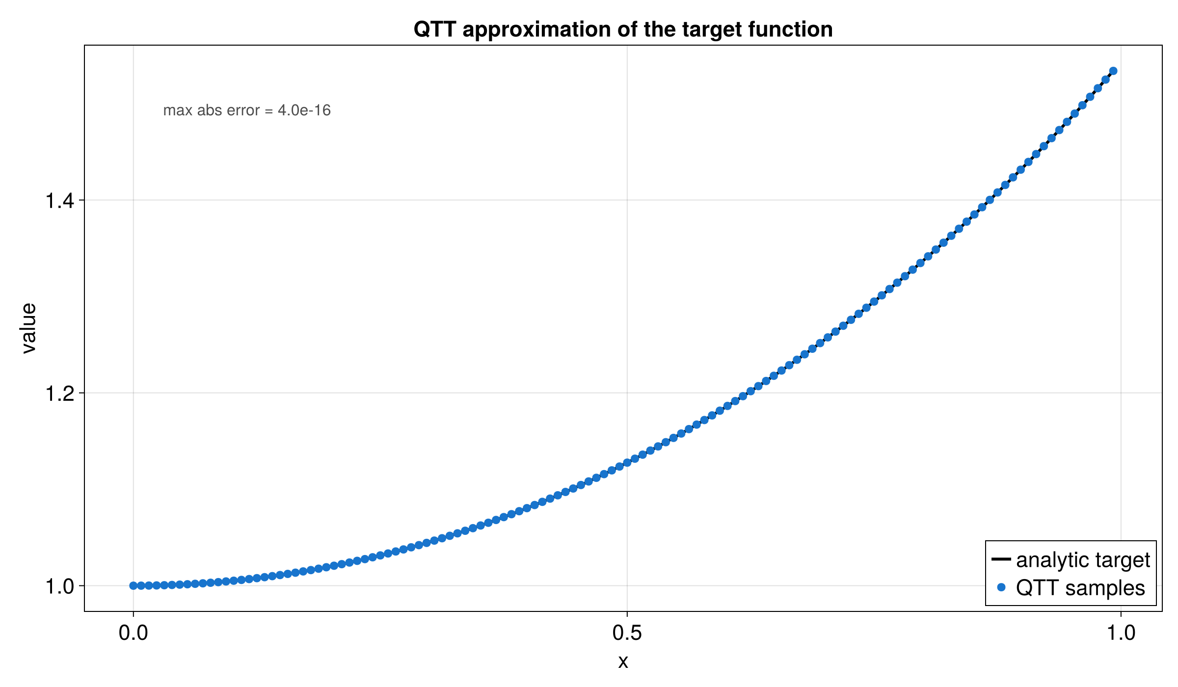
The points from the QTT lie on top of the direct function values. The next plot shows the bond dimensions along the QTT chain. In examples with a visible peak, that peak would mean that part of the grid needs more internal information than its neighbors.

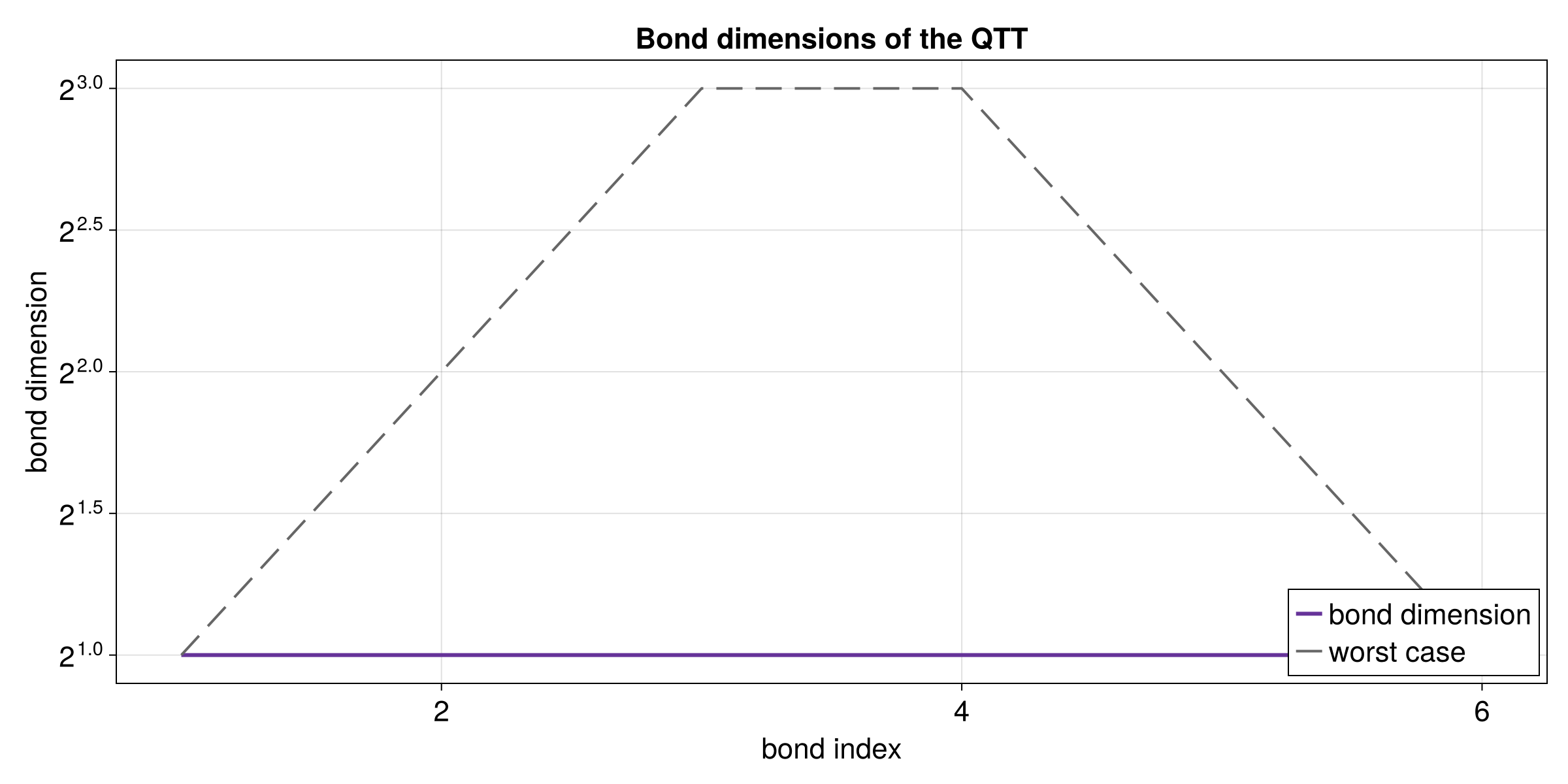
QTT on a Physical Interval

The previous tutorial used integer grid indices. This one maps those indices to a real interval, for example [-1, 2]. That is useful when the function is defined as f(x), not as f(i).

Runnable source: docs/tutorial-code/src/bin/qtt_interval.rs

Key API Pieces

DiscretizedGrid owns the mapping from grid index to physical coordinate. Here the target function is f(x) = x^2 on [-1, 2].

fn main() -> anyhow::Result<()> {
use tensor4all_quanticstci::{
    quanticscrossinterpolate, DiscretizedGrid, QtciOptions, UnfoldingScheme,
};
let grid = DiscretizedGrid::builder(&[7])
    .with_lower_bound(&[-1.0])
    .with_upper_bound(&[2.0])
    .include_endpoint(true)
    .with_unfolding_scheme(UnfoldingScheme::Interleaved)
    .build()?;

let f = |coords: &[f64]| -> f64 {
    let x = coords[0];
    x.powi(2)
};
let options = QtciOptions::default()
    .with_verbosity(0);
let (qtt, _ranks, _errors) = quanticscrossinterpolate(&grid, f, None, options)?;

assert!((qtt.evaluate(&[127])? - 4.0).abs() < 1e-8);
Ok(())
}

Indices passed to evaluate are zero-based grid indices. The grid converts them to the physical coordinate before the function is sampled. Passing None for the optional initial-pivot argument keeps the tutorial on the default QTCI initialization path.

What It Computes

The example builds a DiscretizedGrid, evaluates f(x) = x^2 on that grid, and checks that the QTT follows the direct values on the interval.

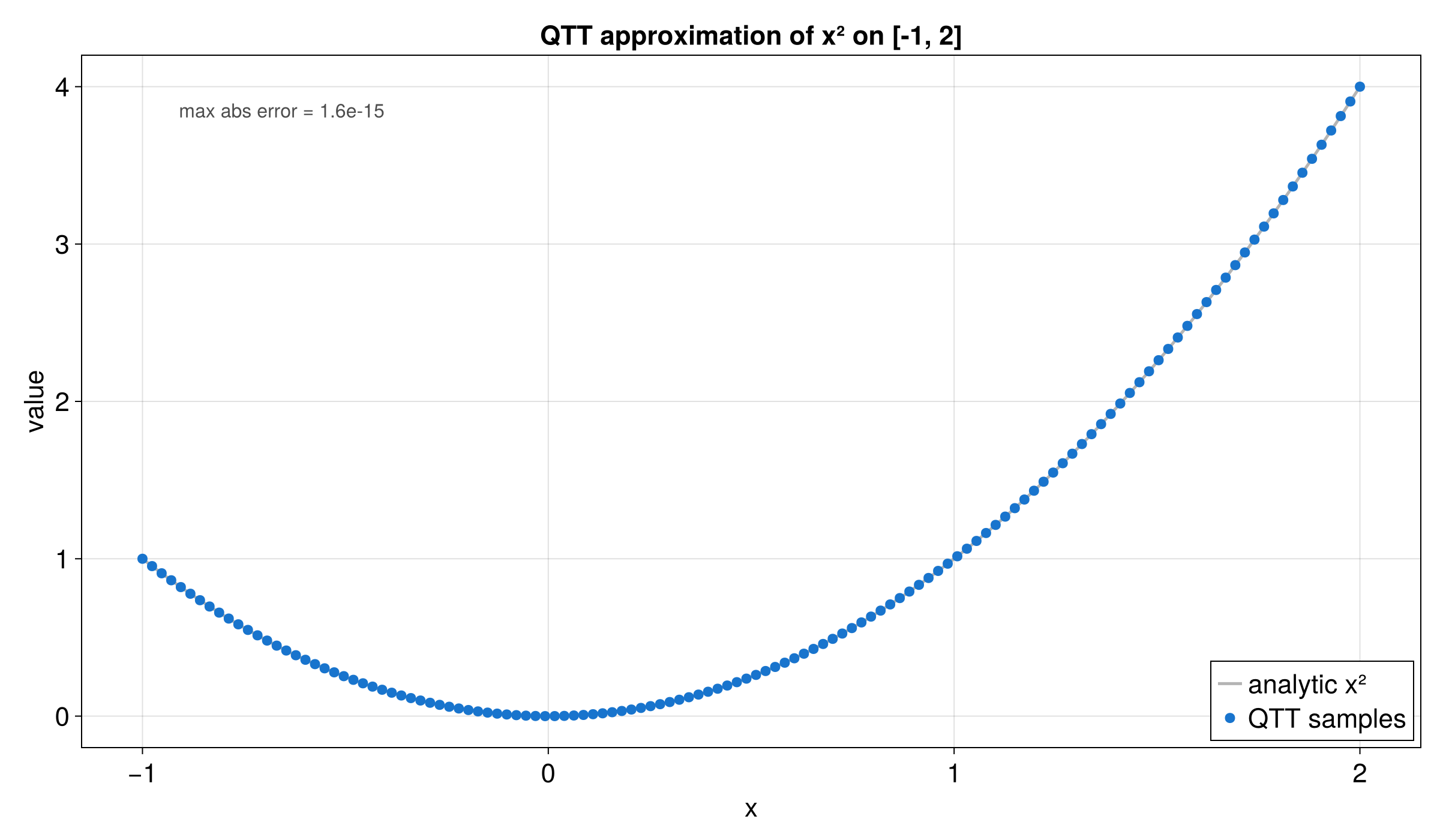
The bond-dimension plot shows how much information is carried between QTT sites. For this smooth example, the internal sizes stay modest.

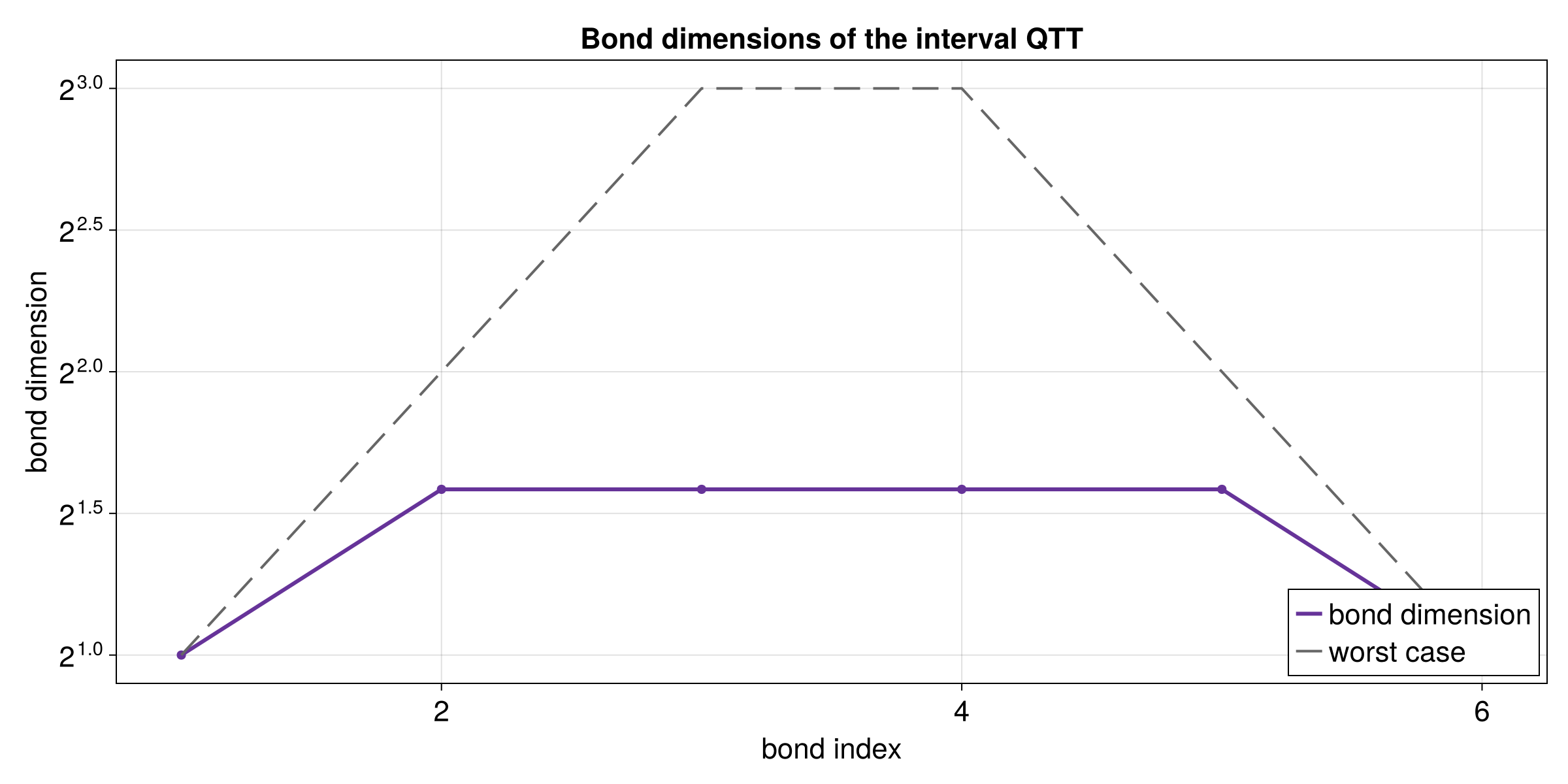
Definite Integrals

After a QTT has been built on a physical interval, it can approximate an integral by summing its grid values and multiplying by the grid spacing. For a smooth function this is a compact way to keep the sampled values and an integral estimate together.

Runnable source: docs/tutorial-code/src/bin/qtt_integral.rs

Key API Pieces

integral() is available when the QTT was built from a DiscretizedGrid. This example uses the same target function as the interval tutorial, f(x) = x^2 on [-1, 2].

fn main() -> anyhow::Result<()> {
use tensor4all_quanticstci::{quanticscrossinterpolate, DiscretizedGrid, QtciOptions};
let grid = DiscretizedGrid::builder(&[7])
    .with_lower_bound(&[-1.0])
    .with_upper_bound(&[2.0])
    .include_endpoint(true)
    .build()?;

let f = |coords: &[f64]| -> f64 {
    let x = coords[0];
    x.powi(2)
};
let options = QtciOptions::default()
    .with_verbosity(0);
let (qtt, _ranks, _errors) = quanticscrossinterpolate(&grid, f, None, options)?;

let integral = qtt.integral()?;
let exact = 3.0;
assert!((integral - exact).abs() < 8e-2);
Ok(())
}

For non-constant functions, compare the result against an analytic integral or a trusted high-resolution reference.

What It Computes

The tutorial builds the same interval QTT as before and calls integral() on it. The plot below comes from the bit-depth sweep and shows how the integral error changes as the grid is refined.

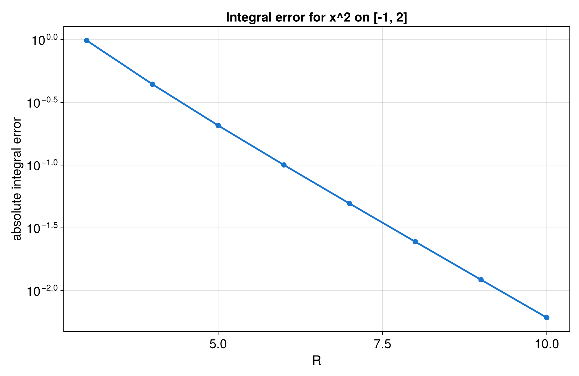
The integral is still a grid approximation. More bits give more grid points, but they can also increase the work needed to build the QTT.

Sweep over Bit Depth

The bit depth R sets the number of grid points: 2^R. Increasing R usually improves resolution, but it may also increase build time or bond dimensions.

Runnable source: docs/tutorial-code/src/bin/qtt_r_sweep.rs

Key API Pieces

The core loop changes only the grid size. The QTCI call stays the same. The target function is f(x) = sin(10x) on the unit interval, with the zero-based discrete grid index mapped to x in [0, 1).

fn main() -> anyhow::Result<()> {
use tensor4all_quanticstci::{quanticscrossinterpolate_discrete, QtciOptions};
let mut point_counts = Vec::new();

for bits in [7usize, 8] {
    let size = 1usize << bits;
    let sizes = [size];
    let target_function = |x: f64| -> f64 { (10.0 * x).sin() };
    let f = move |idx: &[usize]| -> f64 {
        let x = idx[0] as f64 / size as f64;
        target_function(x)
    };
    let options = QtciOptions::default()
        .with_verbosity(0);
    let (qtt, _ranks, _errors) =
        quanticscrossinterpolate_discrete::<f64, _>(&sizes, f, None, options)?;

    let last_grid_index = size - 1;
    let x_last = last_grid_index as f64 / size as f64;
    assert!((qtt.evaluate(&[last_grid_index])? - target_function(x_last)).abs() < 1e-8);
    point_counts.push(size);
}

assert_eq!(point_counts, vec![128, 256]);
Ok(())
}

Use sweeps like this when choosing a grid before running a larger computation.

What It Computes

The example repeats the same QTT construction for several bit depths and writes the value error, runtime, and sample curves.

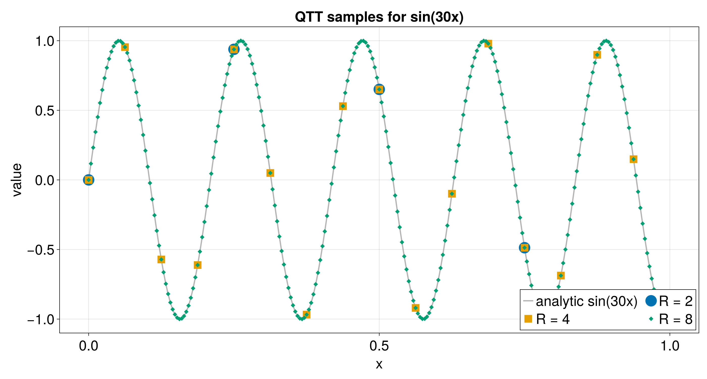
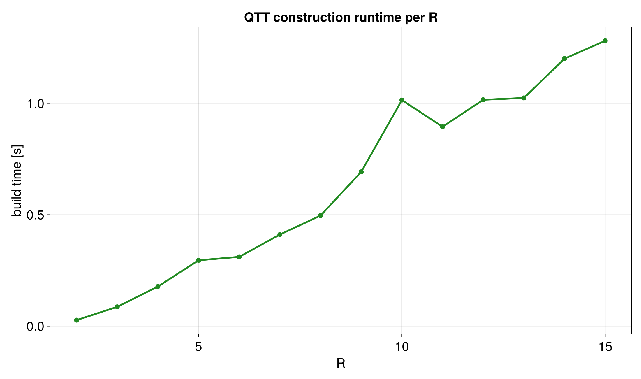
Multivariate Functions

A multivariate QTT stores a function such as f(x, y). The sites can be grouped by variable or interleaved. Grouped means all bits for one variable come first; interleaved means the first bit of each variable appears before the second bit of each variable. The best choice depends on the function.

Runnable source: docs/tutorial-code/src/bin/qtt_multivariate.rs

Key API Pieces

Use one bit-depth entry per variable when building a DiscretizedGrid. The target function is f(x, y) = x * cos(x) * cos(y).

fn main() -> anyhow::Result<()> {
use tensor4all_quanticstci::{
    quanticscrossinterpolate, DiscretizedGrid, QtciOptions, UnfoldingScheme,
};
let grid = DiscretizedGrid::builder(&[7, 7])
    .with_variable_names(&["x", "y"])
    .with_bounds(-2.0, 2.0)
    .include_endpoint(false)
    .with_unfolding_scheme(UnfoldingScheme::Interleaved)
    .build()?;

let f = |coords: &[f64]| -> f64 {
    let x = coords[0];
    let y = coords[1];
    x * x.cos() * y.cos()
};
let options = QtciOptions::default()
    .with_unfoldingscheme(UnfoldingScheme::Interleaved)
    .with_verbosity(0);
let (qtt, _ranks, _errors) = quanticscrossinterpolate(&grid, f, None, options)?;

assert!((qtt.evaluate(&[0, 0])? - f(&[-2.0, -2.0])).abs() < 1e-6);
Ok(())
}

The tutorial binary builds a QTT for f(x, y) = x * cos(x) * cos(y) and compares the two layouts visually.

What It Computes

The example builds a two-dimensional QTT with both layouts and compares the values, errors, and bond dimensions.

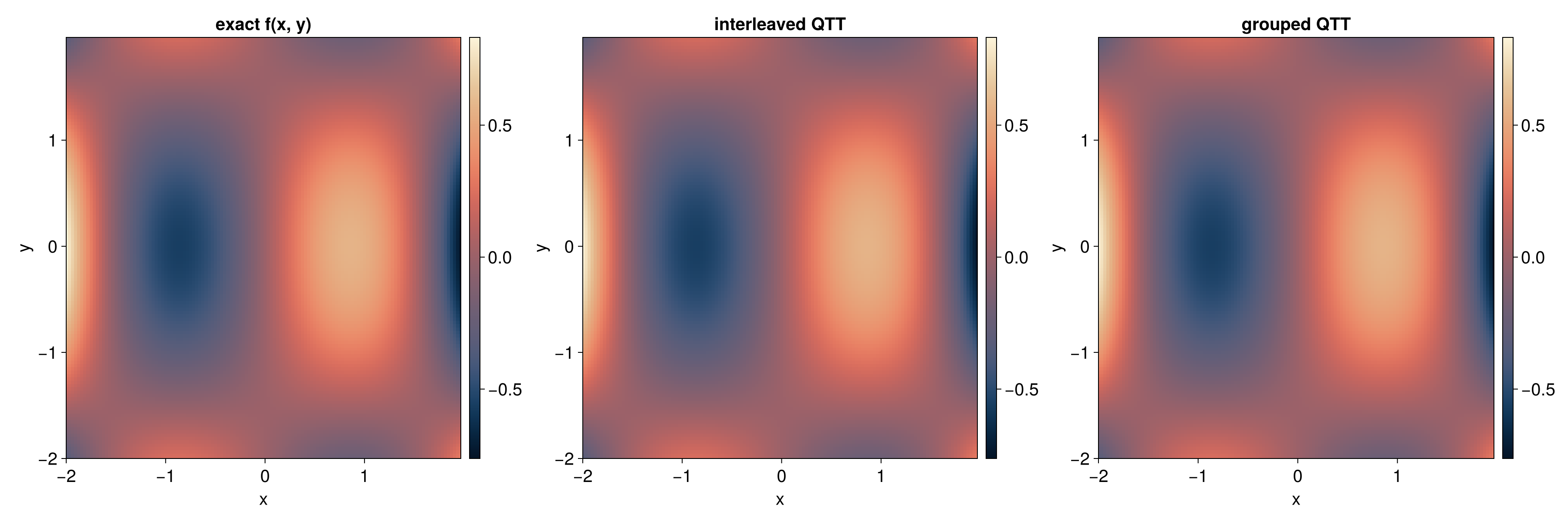
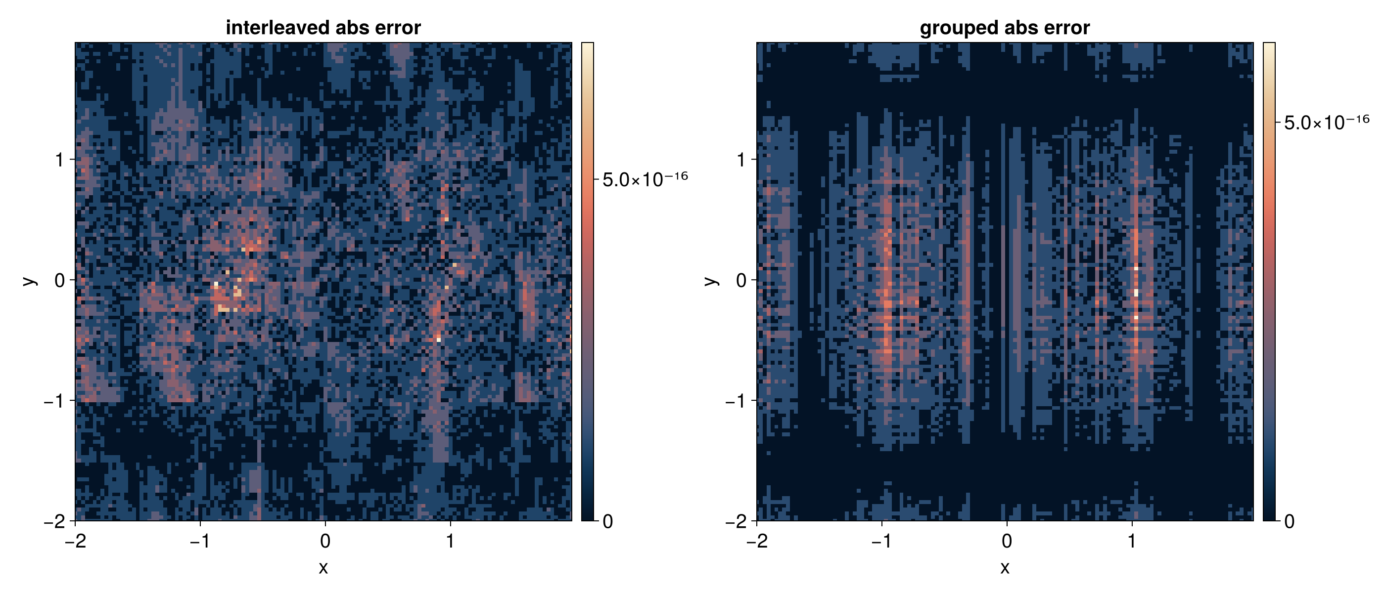
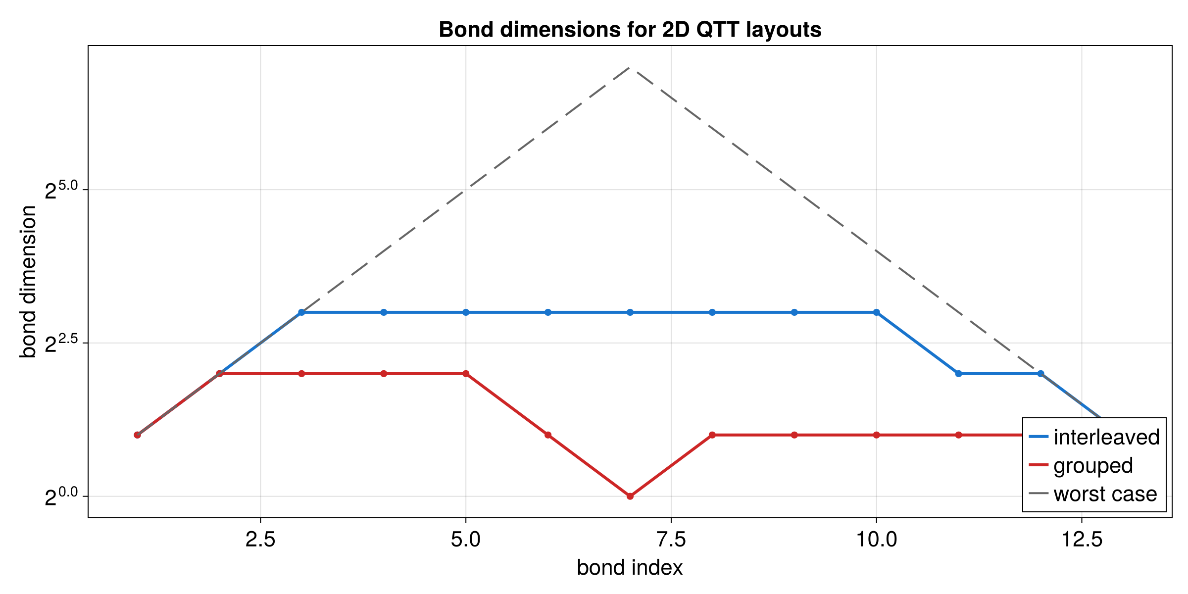
Interpolative QTT

Interpolative QTT builds a tensor train by sampling a function through local Chebyshev-Lobatto interpolation. This is useful when the function is already given on a physical interval and known nonsmooth or sharply localized points should stay on a multiscale refinement path.

Runnable source: docs/tutorial-code/src/bin/interpolative_qtt.rs

Key API Pieces

Use interpolate_single_scale for a smooth one-dimensional function on one interval. The result is a binary SimpleTensorTrain, so the site index [0, 0, ...] evaluates the left endpoint of the sampled interval.

fn main() -> anyhow::Result<()> {
use tensor4all_interpolativeqtt::{
    interpolate_single_scale, AbstractTensorTrain, InterpolativeQttOptions,
};

let options = InterpolativeQttOptions::default().with_tolerance(1e-12);
let tt = interpolate_single_scale(
    |x| (-x * x).exp(),
    -1.0,
    1.0,
    5,
    12,
    &options,
)?;

let value = tt.evaluate(&[0, 0, 0, 0, 0])?;
assert!((value - (-1.0_f64).exp()).abs() < 1e-10);
Ok(())
}

Use interpolate_multi_scale when a known location should remain refined. The following target is a finite, softened version of 1 / r^2; the point x = 0 is still the sharp feature.

fn main() -> anyhow::Result<()> {
use tensor4all_interpolativeqtt::{
    interpolate_multi_scale, AbstractTensorTrain, InterpolativeQttOptions,
};

let epsilon = 0.2_f64;
let inverse_square = |x: f64| 1.0 / (x.abs() + epsilon).powi(2);
let options = InterpolativeQttOptions::default().with_tolerance(1e-12);
let tt = interpolate_multi_scale(
    inverse_square,
    -1.0,
    1.0,
    5,
    16,
    &[0.0],
    &options,
)?;

let value = tt.evaluate(&[0, 0, 0, 0, 0])?;
assert!((value - inverse_square(-1.0)).abs() < 1e-8);
Ok(())
}

The multidimensional constructor fuses all variables at the same bit level. For two variables each site has dimension 4, corresponding to the two binary digits at that level.

fn main() -> anyhow::Result<()> {
use tensor4all_interpolativeqtt::{
    interpolate_multi_scale_nd, AbstractTensorTrain, InterpolativeQttOptions,
};

let epsilon = 0.2_f64;
let radial_inverse_square = |x: &[f64]| {
    1.0 / (x[0] * x[0] + x[1] * x[1] + epsilon * epsilon)
};
let options = InterpolativeQttOptions::default().with_tolerance(1e-12);
let tt = interpolate_multi_scale_nd(
    radial_inverse_square,
    &[-1.0, -1.0],
    &[1.0, 1.0],
    4,
    8,
    &[vec![0.0, 0.0]],
    &options,
)?;

assert_eq!(tt.site_dims(), vec![4, 4, 4, 4]);
let value = tt.evaluate(&[0, 0, 0, 0])?;
assert!((value - radial_inverse_square(&[-1.0, -1.0])).abs() < 1e-8);
Ok(())
}

The tutorial binary runs these three constructions and writes CSV output for the plots below.

What It Computes

The first example uses single-scale interpolation for exp(-x^2). The second uses multiscale interpolation for a softened one-dimensional inverse-square profile, keeping the origin on the refinement path.

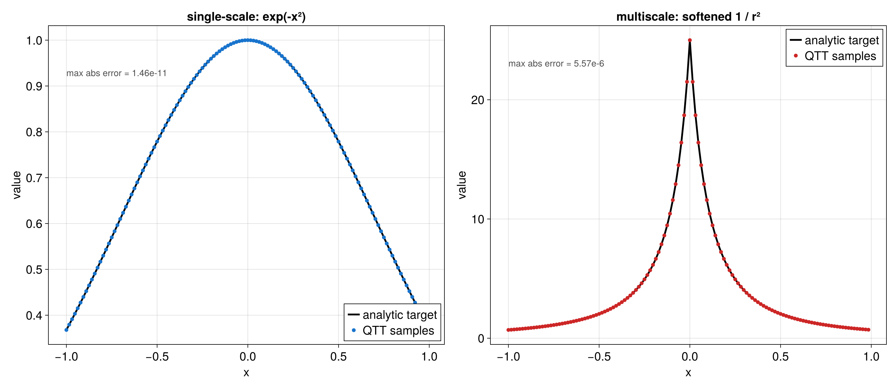
The third example uses interpolate_multi_scale_nd for a two-dimensional softened radial inverse-square profile. The error plot uses log10 absolute error so both the peak and the background remain visible.

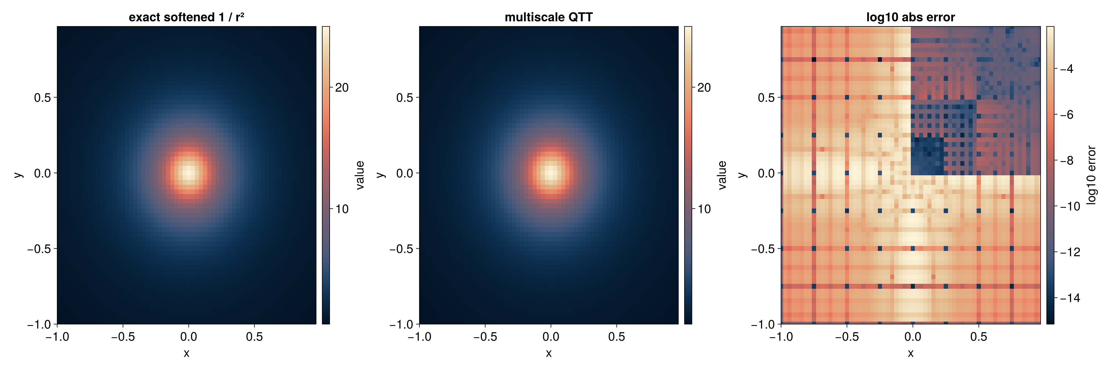
The final plot compares the bond dimensions for all three examples. The multiscale cases need larger internal spaces near the refined point, and the two-dimensional fused sites are more expensive than the one-dimensional sites.

CUDA TreeTN Contraction

This experimental path contracts a small dense TreeTN<IdxTensor> on one NVIDIA GPU. Transfers are explicit: tensor4all-rs never uploads, downloads, or falls back to the CPU inside the contraction.

Prerequisites

• A stable Rust toolchain; see Getting Started.
• An NVIDIA GPU and CUDA driver/toolkit compatible with the CUDA versions used by the pinned tenferro/cubecl dependencies. No wider version or compute-capability support matrix is currently promised.
• The intended device must be visible as CUDA ordinal 0.
• Build with the non-default tenferro-cuda feature. The commands also name the default tenferro-cpu-faer feature explicitly because the quickstart computes a CPU reference alongside the CUDA contraction.

Clone tensor4all-rs and run the checked quickstart:

git clone https://github.com/tensor4all/tensor4all-rs.git
cd tensor4all-rs
cargo run --release -p tensor4all-treetn --example cuda_quickstart \
  --features tenferro-cuda,tenferro-cpu-faer

The complete checked source is embedded below. It is rendered as text rather than an mdBook-tested Rust block because executing it requires CUDA hardware; the feature-gated example itself is compile-checked and run on CUDA.

use std::error::Error;

use tensor4all_core::{CudaExecutionContext, DynIndex, IdxTensor};
use tensor4all_treetn::TreeTN;

fn main() -> Result<(), Box<dyn Error>> {
    let left = DynIndex::new_dyn(2);
    let bond = DynIndex::new_dyn(2);
    let right = DynIndex::new_dyn(2);
    let tree = TreeTN::from_tensors(
        vec![
            IdxTensor::from_dense(vec![left, bond.clone()], vec![1.0_f64, 2.0, 3.0, 4.0])?,
            IdxTensor::from_dense(vec![bond, right], vec![5.0_f64, 6.0, 7.0, 8.0])?,
        ],
        vec![0, 1],
    )?;

    let cpu = tree.contract_to_tensor()?;
    let context = CudaExecutionContext::new()?;
    let resident_tree = tree.upload_cuda(&context)?;
    let resident_result = resident_tree.contract_to_tensor_cuda(&context)?;
    resident_result.validate_cuda_residency(&context)?;
    assert!(resident_result.to_vec::<f64>().is_err());

    let result = resident_result.download(&context)?;
    let residual = result.sub(&cpu)?.maxabs()?;
    assert!(residual <= 1.0e-10, "CUDA/CPU residual: {residual}");
    println!(
        "device={:?} residual_max_abs={residual:.3e}",
        context.device_name()
    );
    Ok(())
}

Source: cuda_quickstart.rs.

It performs this flow:

1. Build a two-node host TreeTN and compute a CPU reference.
2. Create one caller-owned CudaExecutionContext for visible ordinal 0.
3. Upload every node with TreeTN::upload_cuda.
4. Contract all internal bonds with contract_to_tensor_cuda.
5. Verify that the result is still resident in the same CUDA context.
6. Download explicitly and assert a maximum CPU/GPU residual of at most 1e-10.

A successful run prints the GPU name and residual, for example:

device="NVIDIA A100 80GB PCIe" residual_max_abs=0.000e0

Using it from another project

The crates are not published to crates.io yet. Enable CUDA on both crates imported by the quickstart:

[dependencies]
tensor4all-core = { git = "https://github.com/tensor4all/tensor4all-rs", features = ["tenferro-cuda", "tenferro-cpu-faer"] }
tensor4all-treetn = { git = "https://github.com/tensor4all/tensor4all-rs", features = ["tenferro-cuda", "tenferro-cpu-faer"] }

Create a binary project, put the dependency entries above under [dependencies] in Cargo.toml, and copy the embedded program to src/main.rs:

cd ..
cargo new cuda-tree-quickstart
cd cuda-tree-quickstart
# Add the dependency entries above to Cargo.toml.
cp ../tensor4all-rs/crates/tensor4all-treetn/examples/cuda_quickstart.rs src/main.rs
cargo run --release

Keep one CudaExecutionContext for upload, contraction, synchronization, and download. Mixing host and CUDA nodes, CUDA contexts, or node dtypes returns a typed error before contraction; it does not trigger a hidden transfer or CPU fallback.

Current limits

This is a dense full-network contraction, so output memory scales with the product of external-index dimensions. It currently supports only:

• dense, untracked IdxTensor nodes;
• one dtype and one CUDA context across the tree;
• visible CUDA ordinal 0;
• full contraction to one dense tensor.

CUDA SVD, QR, truncation, TreeTN-to-TreeTN contraction, zip-up/fitting, TCI/ACI, automatic device selection, and multi-GPU execution are not yet supported.

For timing, use the separate cuda_tree_contraction example, which reports context setup, upload, warm-up, steady-state GPU contraction plus synchronization, download, and CPU contraction independently:

cargo run --release -p tensor4all-treetn --example cuda_tree_contraction \
  --features tenferro-cuda,tenferro-cpu-faer

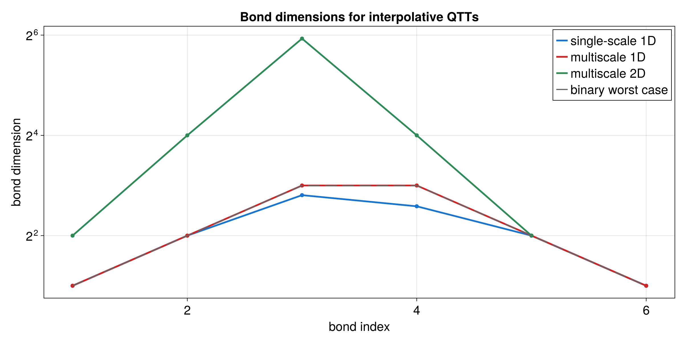
Elementwise Product

This tutorial multiplies two functions after both have been represented as QTTs. Elementwise means that values at the same grid point are multiplied: h(x_i) = f(x_i) g(x_i).

Runnable source: docs/tutorial-code/src/bin/qtt_elementwise_product.rs

Key API Pieces

The first step is simply to build two QTTs on the same grid. Converting to TreeTN enables partial_contract with diagonal_pairs for the pointwise product. The two target functions are f(x) = x^2 and g(x) = sin(10x) on the unit interval.

fn main() -> anyhow::Result<()> {
use tensor4all_quanticstci::{quanticscrossinterpolate_discrete, QtciOptions};
use tensor4all_treetn::{
    contraction::ContractionOptions,
    partial_contract, tensor_train_to_treetn, PartialContractionSpec,
};
let npoints = 8usize;
let sizes = [npoints];
let f = move |idx: &[usize]| -> f64 {
    let x = idx[0] as f64 / npoints as f64;
    x.powi(2)
};
let g = move |idx: &[usize]| -> f64 {
    let x = idx[0] as f64 / npoints as f64;
    (10.0 * x).sin()
};
let options = QtciOptions::default()
    .with_verbosity(0);

let (qtt_a, _, _) = quanticscrossinterpolate_discrete::<f64, _>(
    &sizes, f, None, options.clone(),
)?;
let (qtt_b, _, _) = quanticscrossinterpolate_discrete::<f64, _>(
    &sizes, g, None, options,
)?;

let tt_a = qtt_a.tensor_train();
let tt_b = qtt_b.tensor_train();
let (tn_a, site_indices_a) = tensor_train_to_treetn(&tt_a)?;
let (tn_b, site_indices_b) = tensor_train_to_treetn(&tt_b)?;

let diagonal_pairs: Vec<_> = site_indices_a
    .iter()
    .cloned()
    .zip(site_indices_b.iter().cloned())
    .collect();
let spec = PartialContractionSpec {
    contract_pairs: vec![],
    diagonal_pairs,
    output_order: Some(site_indices_a.clone()),
};
let center = tn_a.node_names()[0];
let product = partial_contract(
    &tn_a, &tn_b, &spec, &center, ContractionOptions::default(),
)?;

let value = product.evaluate_point(&site_indices_a, &[0usize, 1, 1])?;
let x = (4.0 - 1.0) / npoints as f64;
let expected = x.powi(2) * (10.0 * x).sin();
assert!((value.real() - expected).abs() < 1e-8);
assert_eq!(product.node_count(), 3);
Ok(())
}

The important condition is that both QTTs use compatible grids, so that a site in one QTT refers to the same grid bit as the paired site in the other QTT.

What It Computes

The example builds two QTTs, converts them to TreeTN form, pairs matching grid sites, and contracts those pairs via partial_contract to form the product.

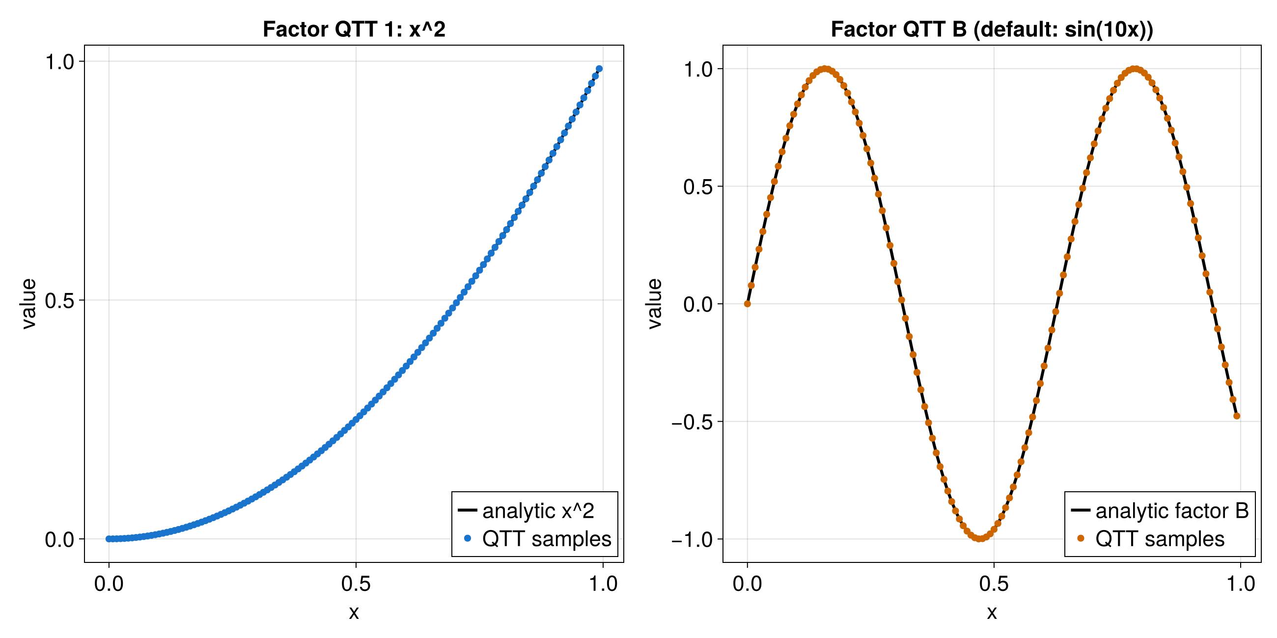
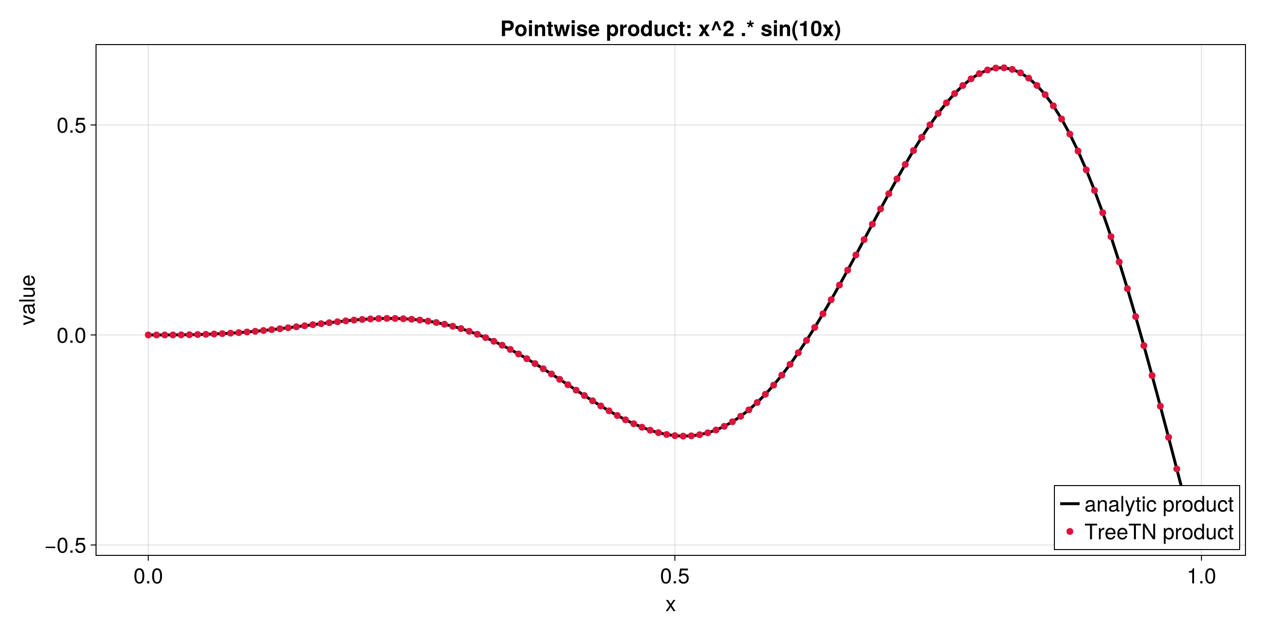
The product may need larger bond dimensions than either factor alone, because it carries information from both inputs.

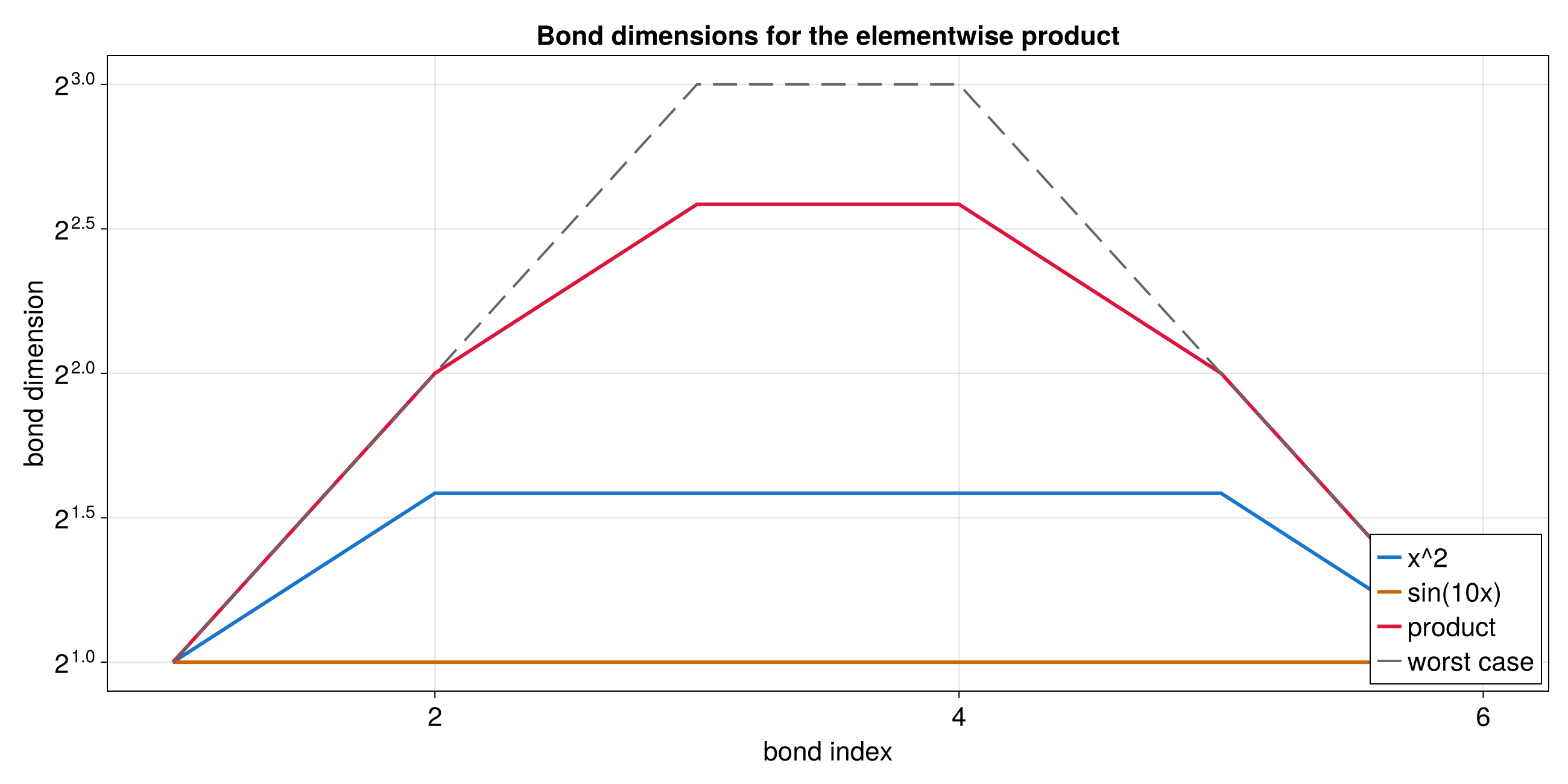
Affine Transformation

An affine transformation evaluates a function at shifted or mixed coordinates. The tutorial uses the pullback point of view: to get the new value at an output point, look up the old function at the transformed input point.

Runnable source: docs/tutorial-code/src/bin/qtt_affine.rs

Key API Pieces

AffineParams stores the matrix and offset. Boundary conditions say what happens when transformed coordinates leave the grid. The operator is applied via tensor_train_to_treetn, align_to_state, and apply_linear_operator. The source function is f(u, v) = sin(2πu/N) + 0.5 cos(2πv/N) + 0.25 sin(2π(u + 2v)/N).

fn main() -> anyhow::Result<()> {
use tensor4all_core::TensorIndex;
use tensor4all_quanticstci::{
    quanticscrossinterpolate_discrete, QtciOptions, UnfoldingScheme,
};
use tensor4all_quanticstransform::{
    affine_operator, AffineParams, BoundaryCondition,
};
use tensor4all_treetn::{apply_linear_operator, tensor_train_to_treetn, ApplyOptions};
use std::f64::consts::PI;

let bits = 7;
let n = 1usize << bits;
let source_grid = [n, n];
let source_function = move |grid_idx: &[usize]| -> f64 {
    let u = grid_idx[0] as f64;
    let v = grid_idx[1] as f64;
    let n = n as f64;
    (2.0 * PI * u / n).sin()
        + 0.5 * (2.0 * PI * v / n).cos()
        + 0.25 * (2.0 * PI * (u + 2.0 * v) / n).sin()
};
let source_options = QtciOptions::default()
    .with_unfoldingscheme(UnfoldingScheme::Fused)
    .with_verbosity(0);

let (source, _, _) = quanticscrossinterpolate_discrete::<f64, _>(
    &source_grid,
    source_function,
    None,
    source_options,
)?;

let params = AffineParams::from_integers(vec![1, 1, 0, 1], vec![0, 0], 2, 2)?;
let mut operator = affine_operator(bits, &params, &[BoundaryCondition::Periodic; 2])?
    .transpose();

let source_tt = source.tensor_train();
let (state, _indices) = tensor_train_to_treetn(&source_tt)?;

operator.align_to_state(&state)?;
let result = apply_linear_operator(&operator, &state, ApplyOptions::naive())?;

let external = TensorIndex::external_indices(&result);
assert_eq!(external.len(), bits);
assert!(result.node_count() >= state.node_count());
Ok(())
}

The full tutorial repeats the same workflow for three boundary conditions. The anti-periodic case uses [AntiPeriodic, Periodic], so only the wrapped u = x + y coordinate changes sign.

What It Computes

The example builds a two-dimensional QTT, creates affine operators, applies them to the QTT, and compares the transformed values with direct references. The anti-periodic pullback matches the periodic wrap except that the region x + y >= N is multiplied by -1.

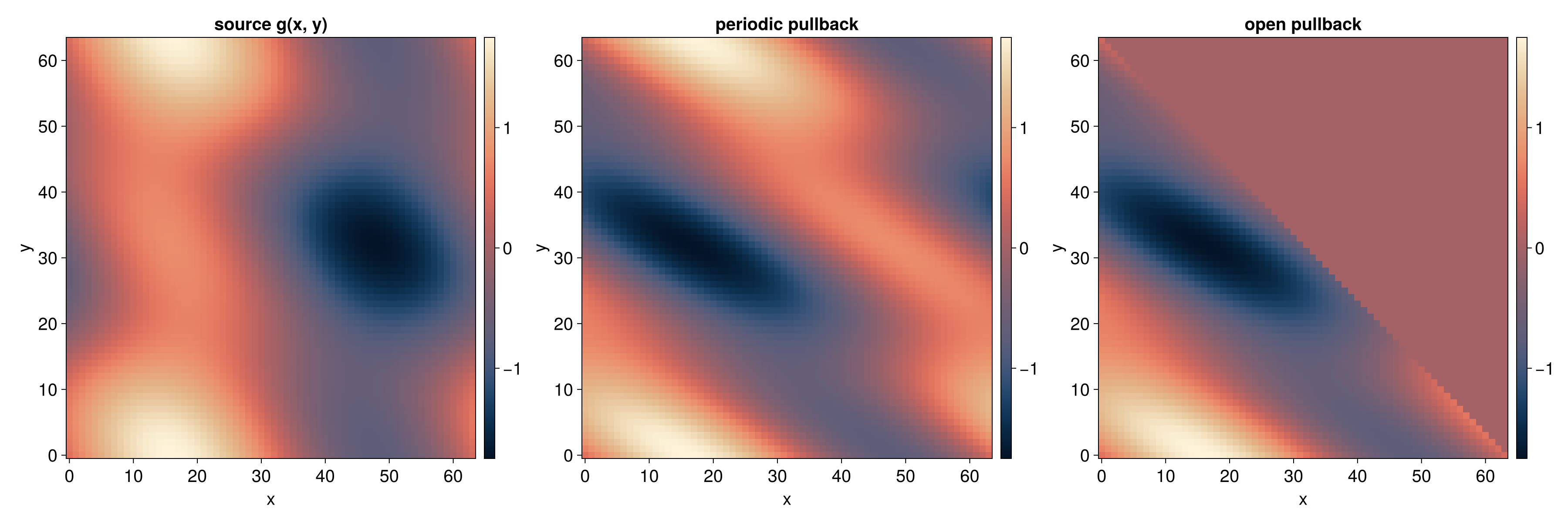
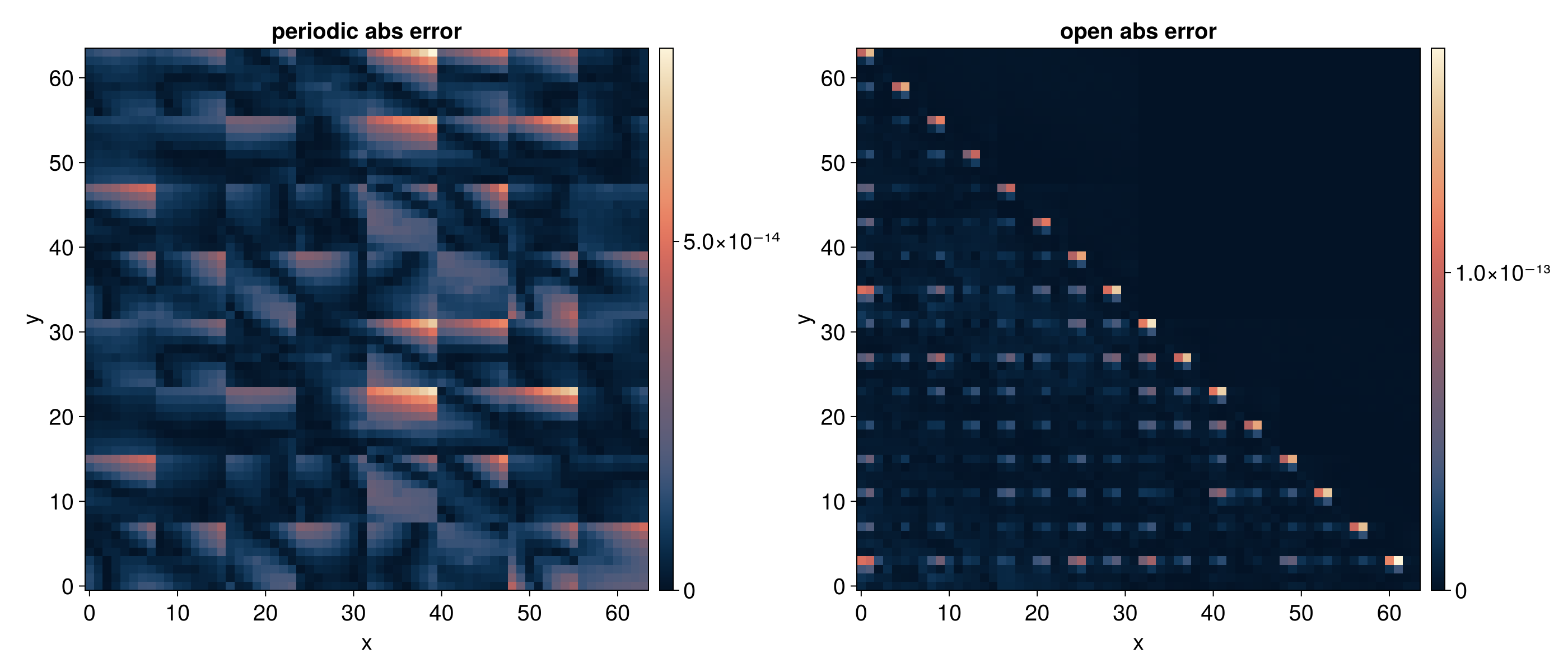
The operator has its own bond dimensions, and the transformed QTT has another set. Both are useful when judging the cost of the operation.

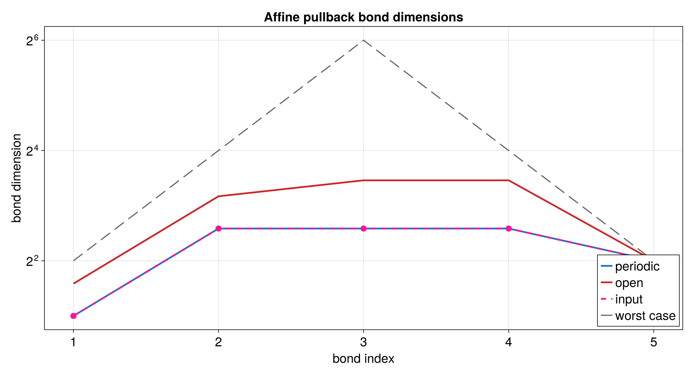
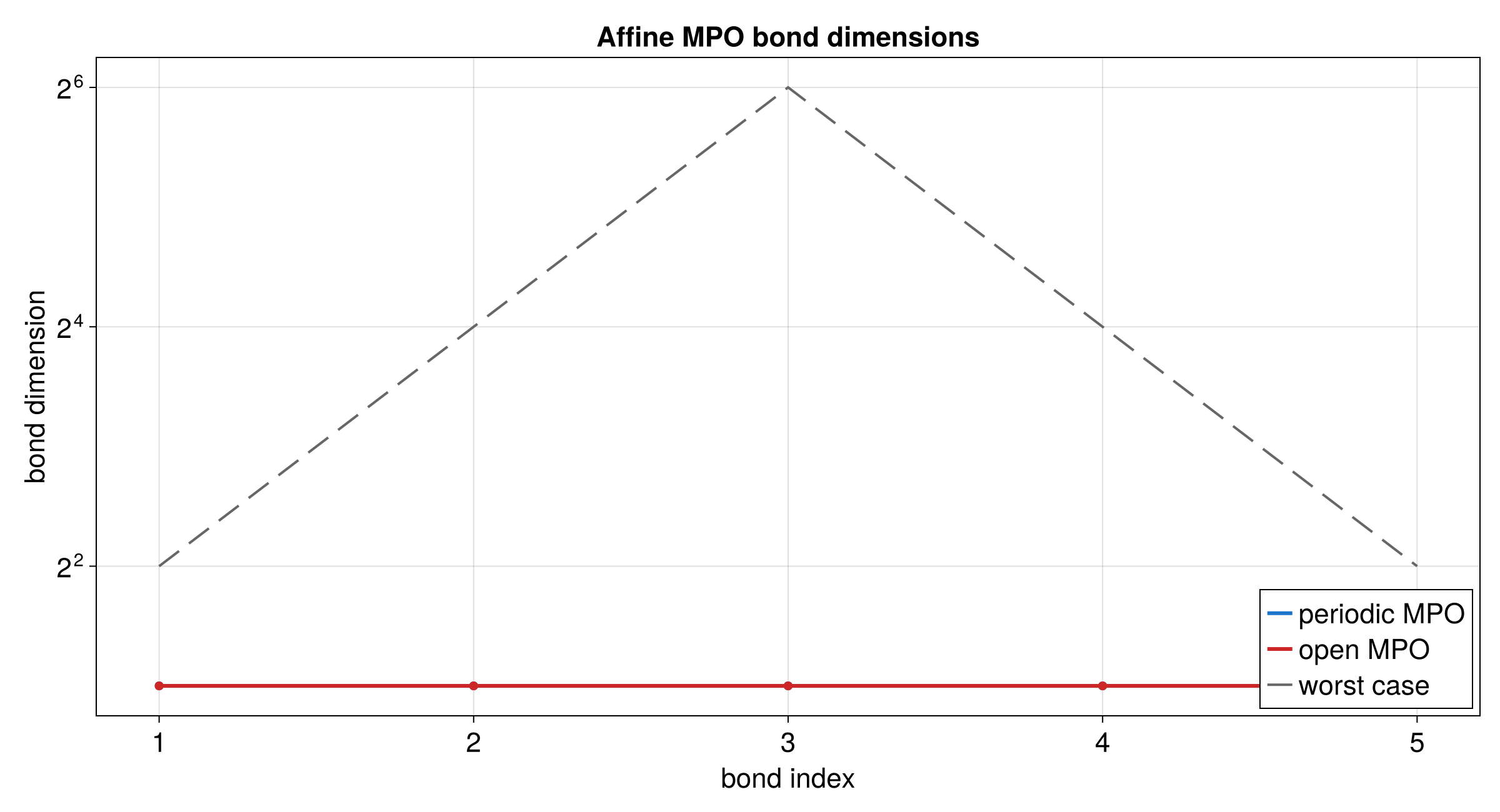
Difference Kernel MPO

A difference kernel is a matrix whose entries depend only on the coordinate difference:

A[x, x'] = f(x - x').

This tutorial starts from a one-dimensional QTT for f(z) and builds the periodic MPO for A[x, x'] = f((x - x') mod 2^R).

Runnable source: docs/tutorial-code/src/bin/qtt_difference_kernel.rs

Key API Pieces

difference_kernel_mpo takes a binary QTT over the difference coordinate and returns an MPO with one fused local index per bit. The local value is encoded as x_bit * 2 + xprime_bit.

fn main() -> anyhow::Result<()> {
use num_complex::Complex64;
use tensor4all_quanticstransform::{difference_kernel_mpo, BoundaryCondition};
use tensor4all_simplett::{AbstractTensorTrain, SimpleTensorTrain};
let bits = 6;
let site_dims = vec![2; bits];

// A real-valued QTT can be converted to Complex64 before calling the transform.
// This compact example uses a constant kernel QTT.
let f = SimpleTensorTrain::constant(&site_dims, Complex64::new(1.0, 0.0));

let mpo = difference_kernel_mpo(&f, BoundaryCondition::Periodic)?;
assert_eq!(mpo.len(), bits);
assert_eq!(mpo.site_dims(), vec![4; bits]);
Ok(())
}

For BoundaryCondition::AntiPeriodic, the same API multiplies entries with x < x' by -1. The checked-in tutorial data uses the periodic case only.

What It Computes

The example builds a smooth periodic source kernel

f(z) = exp(2(cos(2πz/N) - 1))

with N = 2^R, converts the real QTT cores to Complex64, and calls difference_kernel_mpo. The resulting MPO is sampled densely and compared with the direct reference f((x - x') mod N).

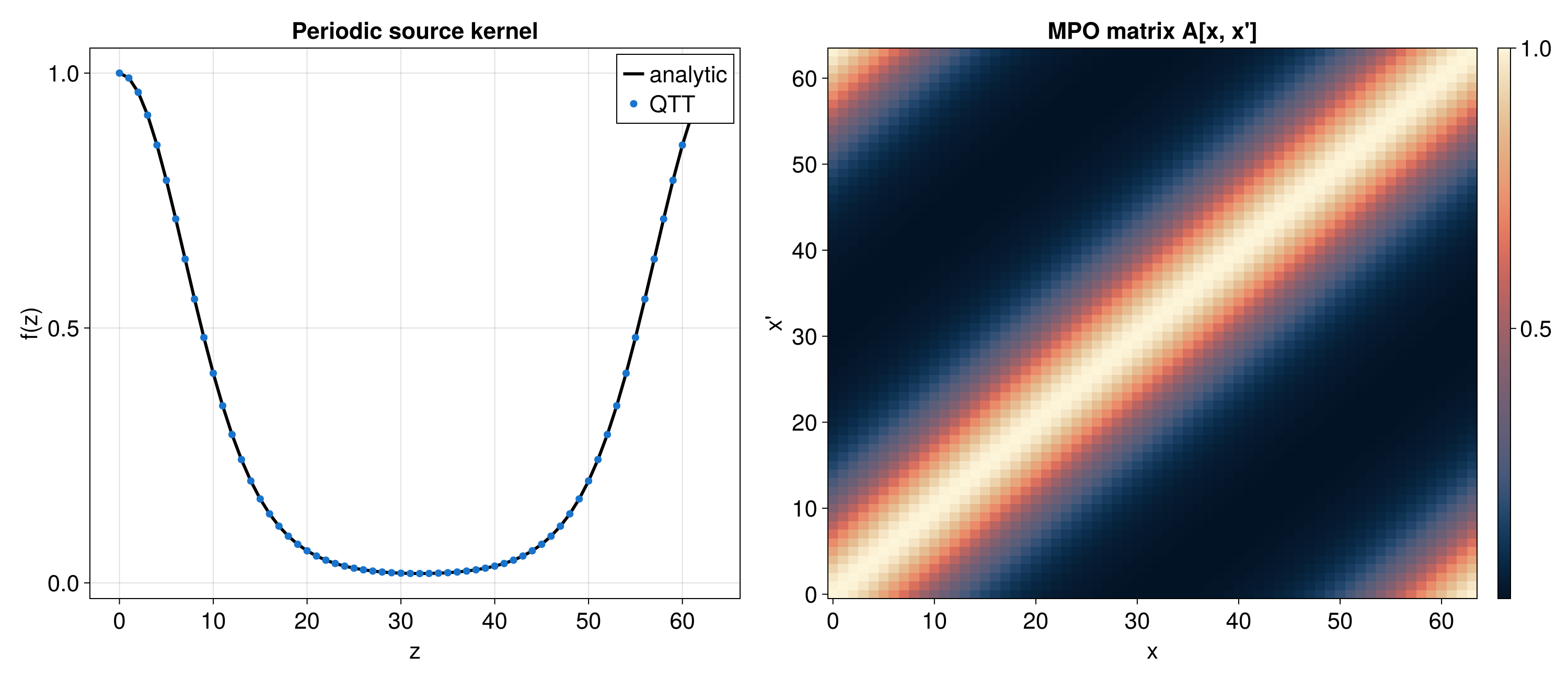
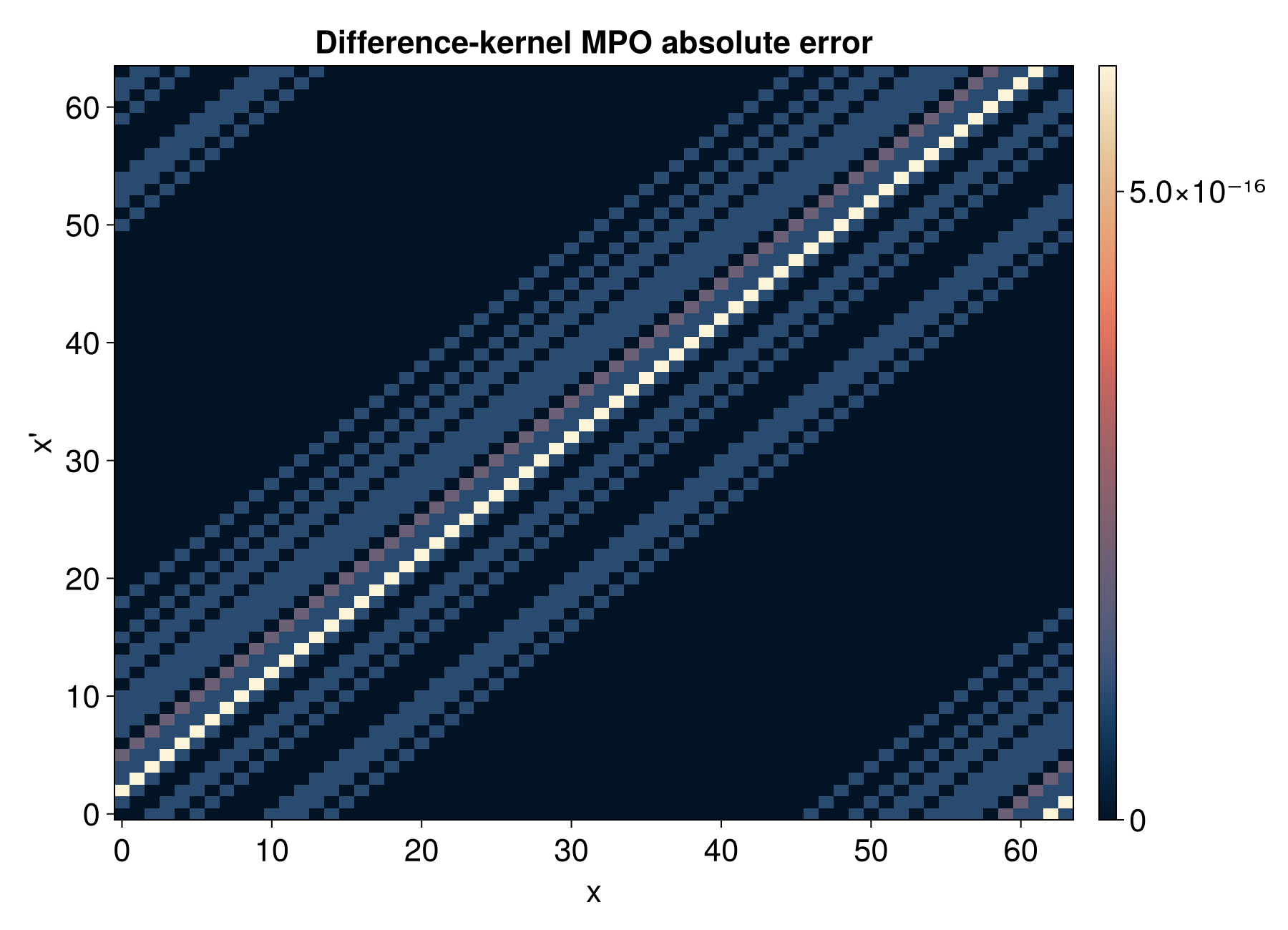
The MPO bonds combine the two-state carry network for x - x' with the source kernel QTT bonds, so the practical bond dimensions are bounded by twice the kernel QTT bond dimensions before any later compression.

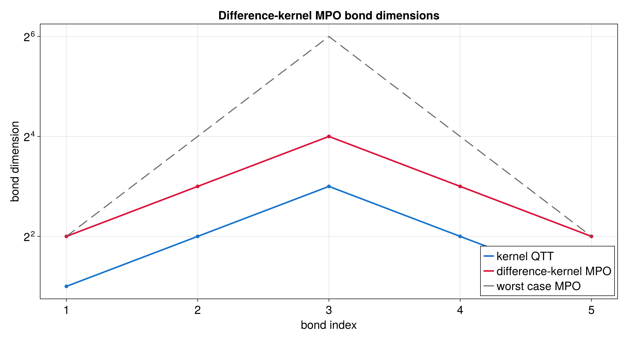
Fourier Transform

This tutorial applies the quantics Fourier operator to a QTT representation of a Gaussian. A Gaussian is a helpful first check because its Fourier transform is also a Gaussian, so the result has a simple reference.

Runnable source: docs/tutorial-code/src/bin/qtt_fourier.rs

Key API Pieces

quantics_fourier_operator creates the operator. The tutorial binary then converts the state to TreeTN, aligns site indices, and applies it via apply_linear_operator. The input target function is the standard Gaussian f(x) = exp(-x^2 / 2).

fn main() -> anyhow::Result<()> {
use tensor4all_quanticstci::{
    quanticscrossinterpolate, DiscretizedGrid, QtciOptions, UnfoldingScheme,
};
use tensor4all_quanticstransform::{quantics_fourier_operator, FourierOptions};
use tensor4all_treetn::{apply_linear_operator, tensor_train_to_treetn, ApplyOptions};
let bits = 7;
let grid = DiscretizedGrid::builder(&[bits])
    .with_lower_bound(&[-10.0])
    .with_upper_bound(&[10.0])
    .include_endpoint(true)
    .with_unfolding_scheme(UnfoldingScheme::Interleaved)
    .build()?;
let gaussian = |coords: &[f64]| -> f64 {
    let x = coords[0];
    (-0.5 * x * x).exp()
};
let options = QtciOptions::default()
    .with_unfoldingscheme(UnfoldingScheme::Interleaved)
    .with_verbosity(0);

let (state, _, _) = quanticscrossinterpolate(&grid, gaussian, None, options)?;

let mut operator = quantics_fourier_operator(bits, FourierOptions::forward())?;
assert_eq!(operator.mpo().node_count(), bits);

let tt = state.tensor_train();
let (state_tn, _indices) = tensor_train_to_treetn(&tt)?;

operator.align_to_state(&state_tn)?;
let result = apply_linear_operator(&operator, &state_tn, ApplyOptions::naive())?;

assert_eq!(result.node_count(), bits);
Ok(())
}

The plotted frequency axis is scaled back to physical units, so the curve can be compared with the analytic Gaussian transform. The quantics Fourier operator follows the bit-reversed output convention described in the Quantum Fourier Transform guide.

What It Computes

The example builds a QTT for the input Gaussian, applies the Fourier operator, and compares selected output values with the analytic transform.

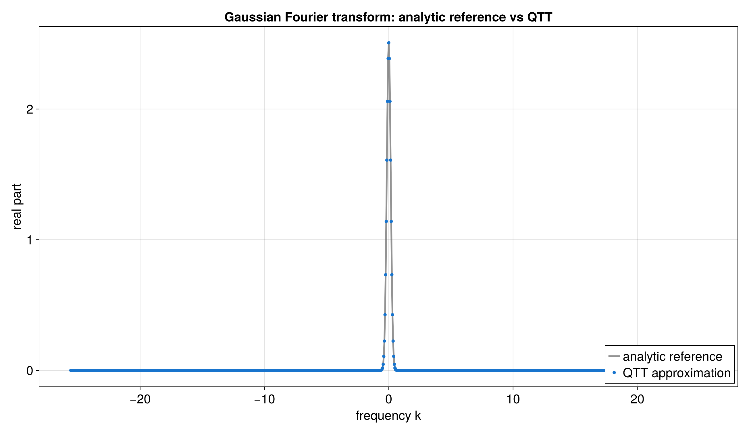
The next plots show the bond dimensions for the input QTT and the operator. The operator dimensions are part of the cost of applying the transform.

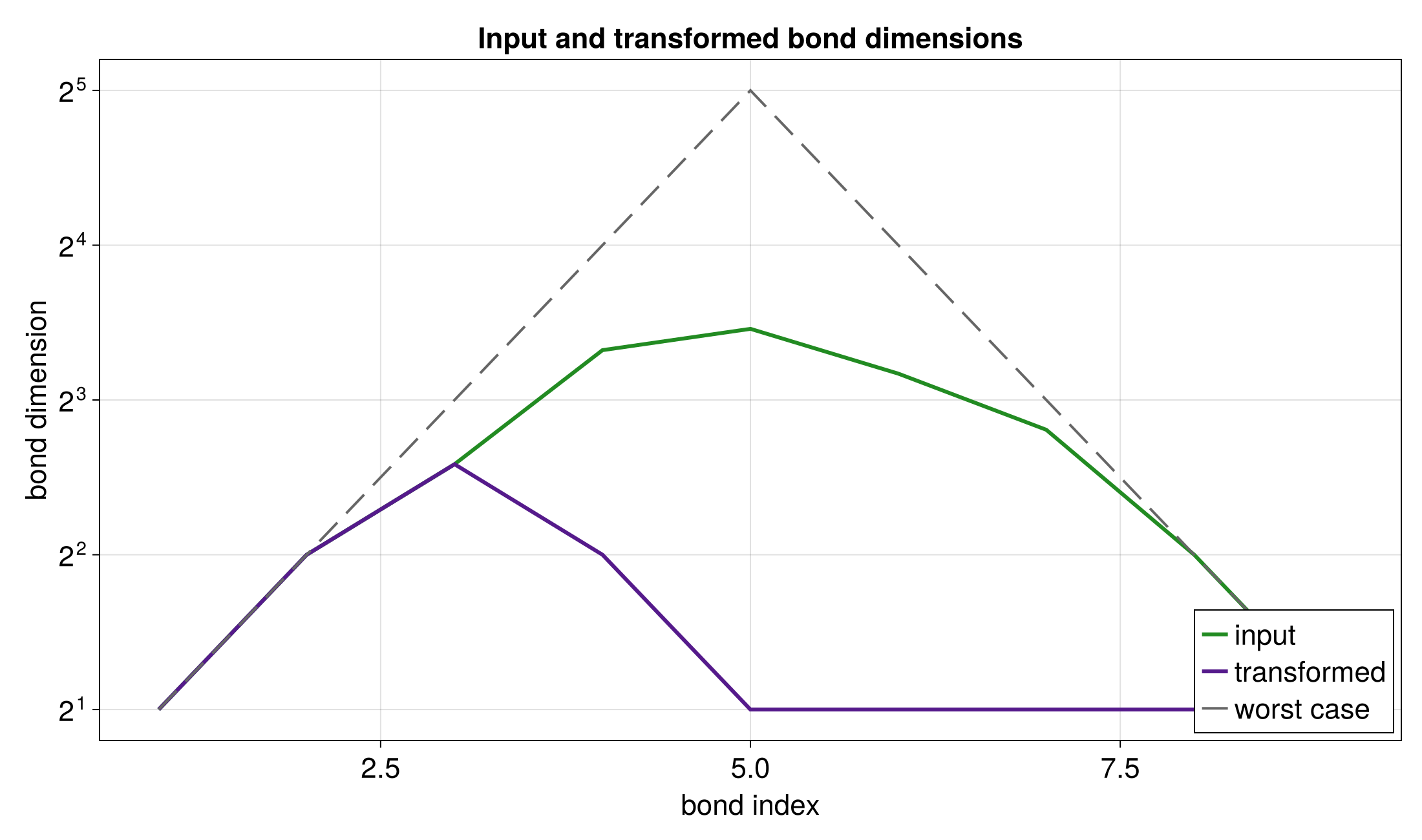
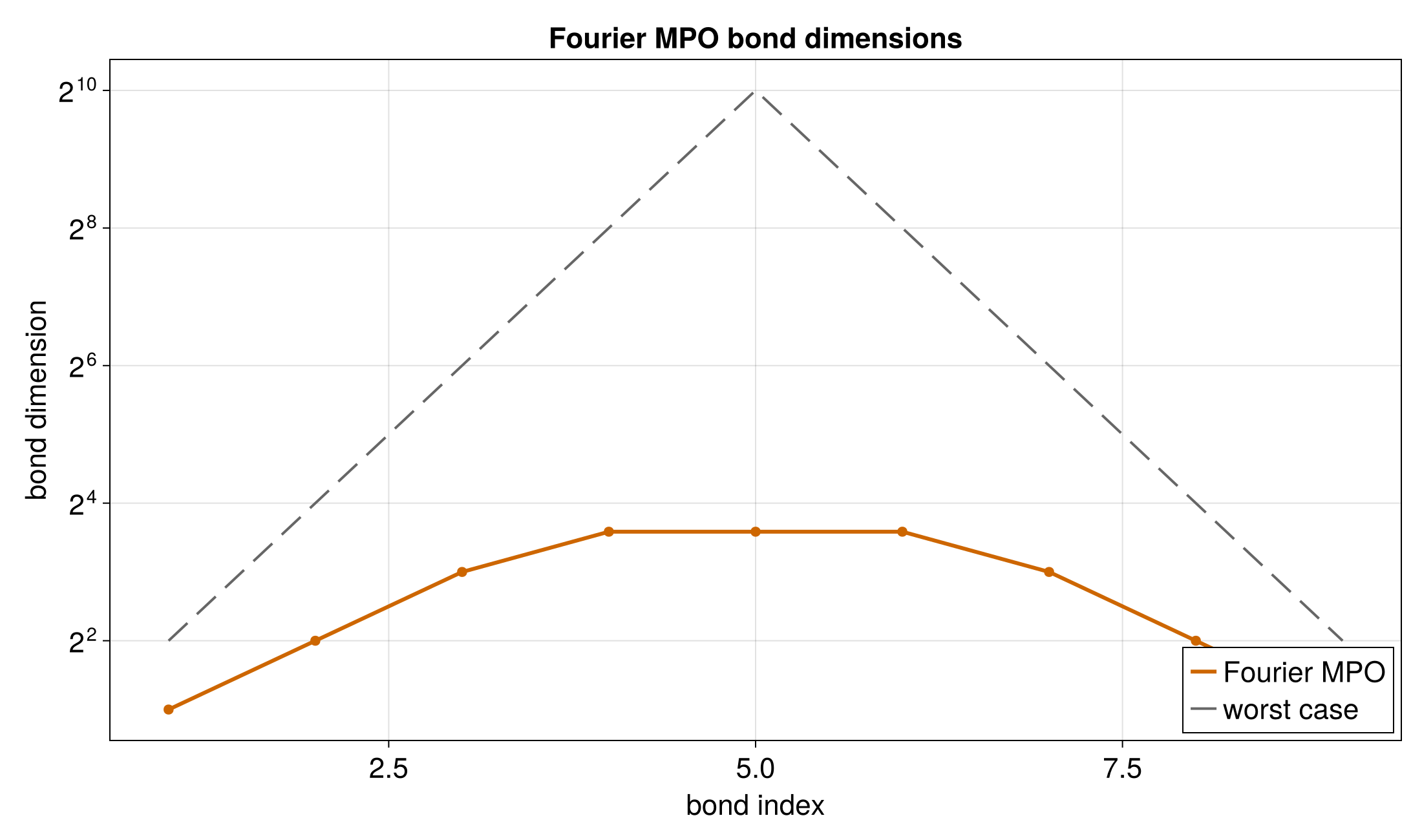
2D Partial Fourier Transform

A partial Fourier transform applies Fourier only along one coordinate of a multivariate function. Here the function is f(x, t), and only the x direction is transformed. The t direction passes through unchanged.

Runnable source: docs/tutorial-code/src/bin/qtt_partial_fourier2d.rs

Key API Pieces

For an interleaved two-variable QTT, the state nodes are ordered x0, t0, x1, t1, .... A one-dimensional Fourier MPO has only x nodes, so the operator nodes are renamed onto the even state nodes. apply_linear_operator then handles the partial operator and leaves the missing t nodes as identity gaps. The source function is f(x, t) = exp(-x^2 / 2) * cos(2πt).

fn main() -> anyhow::Result<()> {
use tensor4all_quanticstci::{
    quanticscrossinterpolate, DiscretizedGrid, QtciOptions, UnfoldingScheme,
};
use tensor4all_quanticstransform::{quantics_fourier_operator, FourierOptions};
use tensor4all_simplett::AbstractTensorTrain;
let bits = 7;
let grid = DiscretizedGrid::builder(&[bits, bits])
    .with_variable_names(&["x", "t"])
    .with_lower_bound(&[-4.0, 0.0])
    .with_upper_bound(&[4.0, 1.0])
    .include_endpoint(true)
    .with_unfolding_scheme(UnfoldingScheme::Interleaved)
    .build()?;

let f = |coords: &[f64]| -> f64 {
    let x = coords[0];
    let t = coords[1];
    (-0.5 * x * x).exp() * (2.0 * std::f64::consts::PI * t).cos()
};
let options = QtciOptions::default()
    .with_unfoldingscheme(UnfoldingScheme::Interleaved)
    .with_verbosity(0);

let (state, _ranks, _errors) = quanticscrossinterpolate(&grid, f, None, options)?;

let operator = quantics_fourier_operator(bits, FourierOptions::forward())?;
assert_eq!(operator.mpo().node_count(), bits);

let x_site_mapping: Vec<_> = (0..bits).map(|site| (site, 2 * site)).collect();
let renamed_operator = operator.rename_nodes(&x_site_mapping)?;

assert_eq!(state.tensor_train().len(), 2 * bits);
assert_eq!(x_site_mapping.len(), bits);
assert_eq!(x_site_mapping[0], (0, 0));
assert_eq!(x_site_mapping[bits - 1], (bits - 1, 2 * (bits - 1)));
assert_eq!(renamed_operator.mpo().node_count(), bits);
Ok(())
}

The full source then aligns the renamed partial operator to the state and applies it. Passing None for initial_pivots is the best starting point for tutorial code because it keeps QTCI on its default initialization path. Explicit pivot lists are a later tuning tool for cases where you already know important grid points. Use apply_linear_operator_to_numbered_tags if and only if numbered tags such as x=1, x=2, … are the intended operator binding.

What It Computes

The example builds an interleaved two-dimensional QTT, applies a one-dimensional Fourier operator to the x-sites, and compares the result with an analytic partial transform.

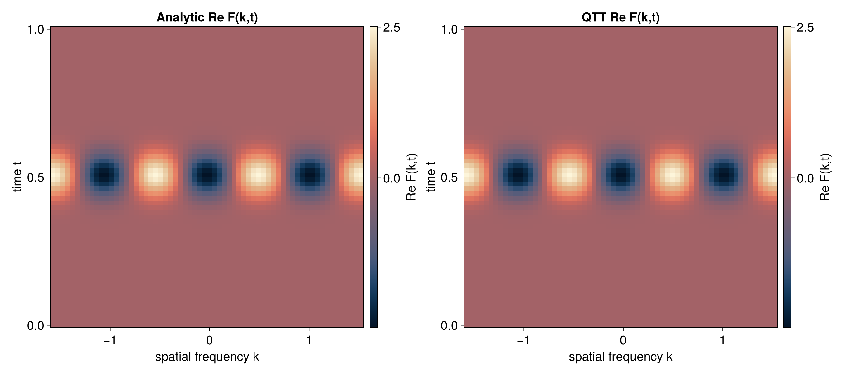
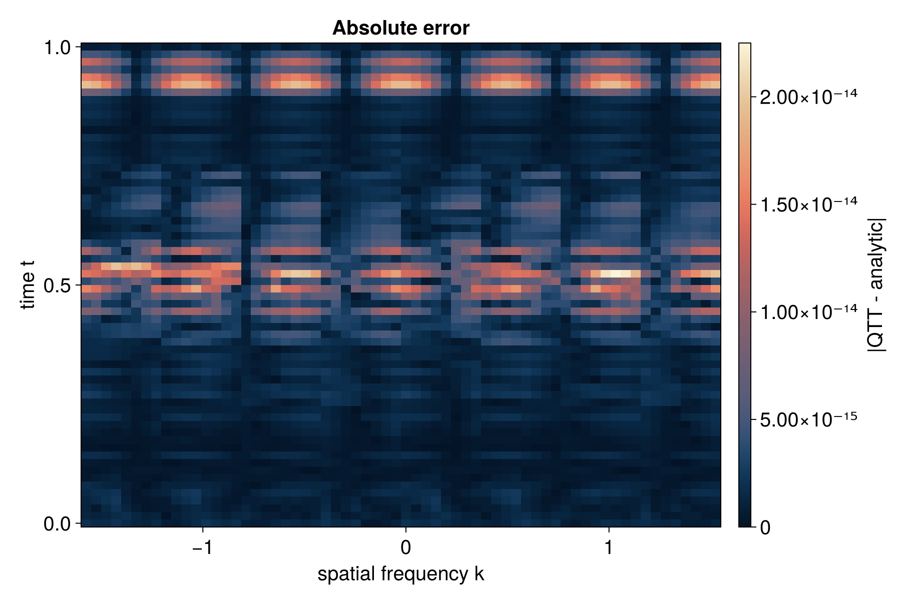
Only the x-sites receive the operator, so the implementation maps the one-dimensional operator nodes onto the even nodes of the interleaved state and lets partial apply supply the identity behavior on the t-sites.

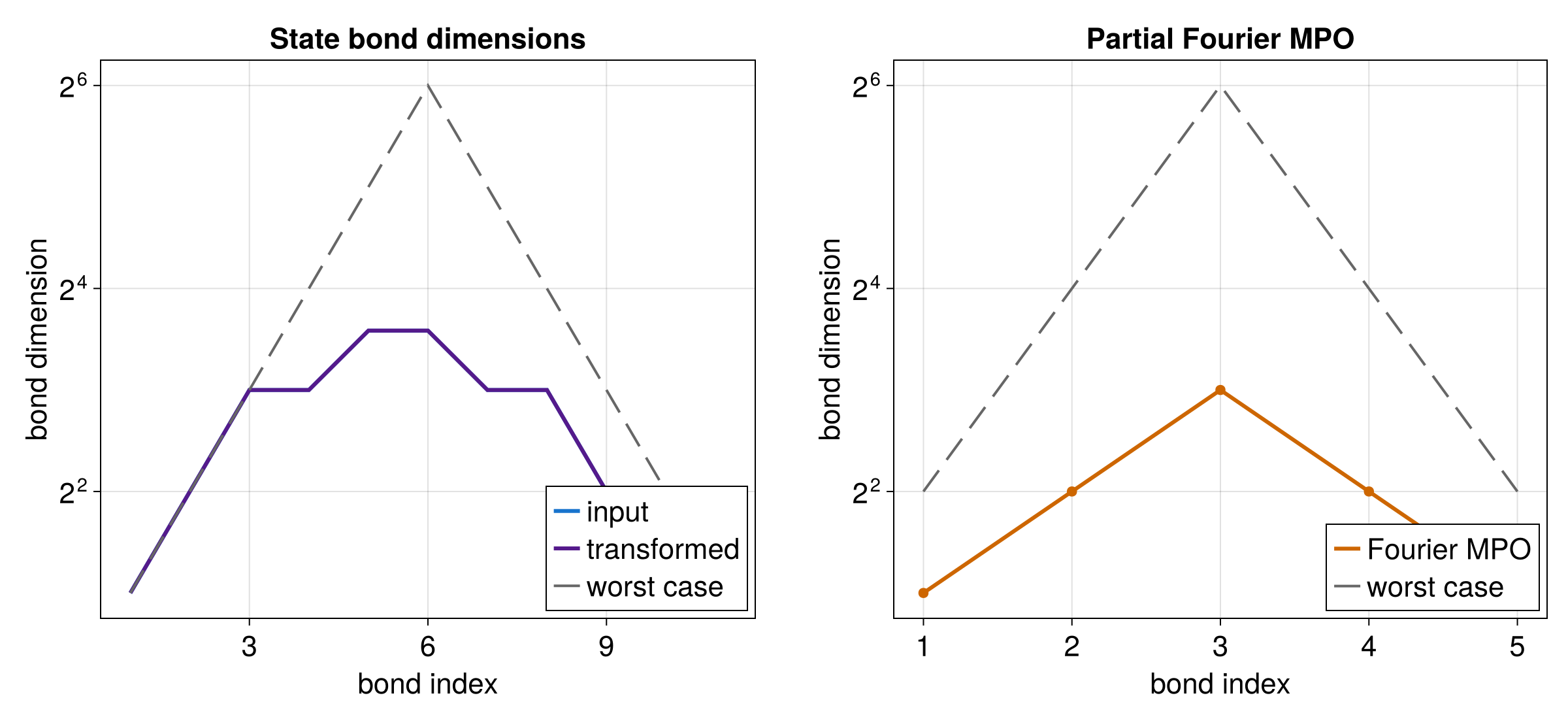
Conventions

This page collects important conventions that apply across the entire tensor4all-rs codebase.

Dense Layout (Column-Major)

tensor4all-rs uses column-major (Fortran order) dense linearization internally. Flat dense buffers, reshape/flatten semantics, the C API, and the HDF5 layer are all defined in terms of column-major ordering.

This matches Julia, ITensors.jl, and tenferro-rs. When exchanging dense data with NumPy, use order="F" when you need explicit control over flattening or reshaping.

Indexing

• Sites and grid indices are 0-indexed in Rust (unlike ITensors.jl, which is 1-indexed). QuanticsTCI.jl scripts must subtract 1 from grid indices at the call boundary.

Truncation Tolerance

tensor4all-rs uses rtol (relative tolerance). ITensors.jl uses cutoff. The conversion is:

rtol = sqrt(cutoff)

Example: ITensors.jl cutoff=1e-10 corresponds to rtol=1e-5 in tensor4all-rs.

Exception — partitioned TreeTNs. tensor4all-partitionedtreetn’s adaptive surface (PatchingOptions::cutoff, truncate_adaptive) follows ITensors.jl cutoff directly: it is a local discarded-weight cutoff, 1:1 with ITensors cutoff (for a caller migrating from the old root-relative value, cutoff = old_rtol², equivalently rtol = sqrt(cutoff)). The final whole-network error is best effort and is not bounded by cutoff; max_bond_dim is the hard cap. The deprecated tensor4all-partitionedtt crate keeps the rtol convention documented above.

Bond-Dimension Cap

tensor4all-rs uses one spelling and one type for the bond-dimension cap across all crates: max_bond_dim: Option<usize> (None = unlimited). No usize::MAX sentinel is used.

maxdim is the closest ITensors.jl cousin of max_bond_dim (bond dimension is the unambiguous tensor-network term; “rank” is overloaded in TCI context).

ITensors.jl Type Correspondence

Scalar Types

IdxTensor supports four scalar types:

• f32 — single-precision real
• f64 — double-precision real
• Complex32 — single-precision complex
• Complex64 — double-precision complex (from the num-complex crate)

Generic APIs handle all four types. Compact Storage snapshots are limited to f64/Complex64; 32-bit tensors retain eager payloads rather than silently promoting their values. Prefer generic code over scalar-specific variants (*_f64 / *_c64) in library and test code. The C API uses scalar-specific names at the FFI boundary where generic dispatch is not available.

Julia Bindings

The Julia bindings for tensor4all-rs are maintained in a separate repository: Tensor4all.jl.

Installation

To install Tensor4all.jl, use Julia’s package manager:

using Pkg
Pkg.add(url="https://github.com/tensor4all/Tensor4all.jl")

This will automatically download and build the Rust library via the C API (tensor4all-capi).

Overview

The current C ABI is intentionally smaller than the full Rust workspace. It exposes the pieces needed to build a Julia-native surface on top:

• Indices — immutable index handles with IDs, tags, and prime levels
• Dense tensors — Float64 / complex tensor construction, export, and contraction
• Tree tensor networks — topology queries, orthogonalization, truncation, evaluation, and dense export
• Canonical QTT layouts — interleaved and fused binary layouts
• Quantics transform materialization — shift, flip, phase rotation, cumsum, Fourier, and affine operators materialized directly as TreeTN
• Error reporting — enum t4a_status_code plus t4a_last_error_message

This split is deliberate: the Rust side owns performance-critical kernels and the Julia side owns higher-level ergonomics.

ABI Conventions

The C API follows Julia-friendly conventions:

• Dense buffers are column-major
• Complex values are interleaved Float64 pairs
• Variable-length outputs use a query-then-fill pattern
• Opaque handles must be released explicitly

The generated public header lives at crates/tensor4all-capi/include/tensor4all_capi.h.

Documentation

For Julia-side examples and package-level documentation, see the Tensor4all.jl README.

For ABI details in this repository, see:

• docs/CAPI_DESIGN.md
• crates/tensor4all-capi/include/tensor4all_capi.h

Linking Rust and Julia Code

If you want to use tensor4all-rs directly in a Rust project and interoperate with Julia, build against the generated C header and follow the conventions documented in docs/CAPI_DESIGN.md.