QTT of a Scalar Function

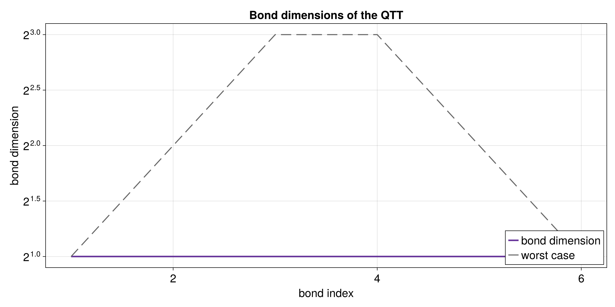
This tutorial builds a quantics tensor train (QTT) for one scalar function on a small binary grid. A QTT stores the values on 2^R grid points as R small sites. The bond dimensions are the internal sizes between neighboring sites; larger values can carry more information but cost more memory and time.

Runnable source: docs/tutorial-code/src/bin/qtt_function.rs

Key API Pieces

Use quanticscrossinterpolate_discrete when the function is most naturally written in terms of grid indices.

fn main() -> anyhow::Result<()> {
use tensor4all_quanticstci::{
    quanticscrossinterpolate_discrete, QtciOptions, UnfoldingScheme,
};
let npoints = 128usize;
let sizes = [npoints];
let f = move |idx: &[i64]| -> f64 {
    let x = (idx[0] as f64 - 1.0) / npoints as f64;
    x.cosh()
};
let options = QtciOptions::default()
    .with_unfoldingscheme(UnfoldingScheme::Interleaved)
    .with_verbosity(0);

let (qtt, ranks, _errors) =
    quanticscrossinterpolate_discrete::<f64, _>(&sizes, f, None, options)?;

let x = 0.5_f64;
assert!((qtt.evaluate(&[65])? - x.cosh()).abs() < 1e-8);
assert!(!ranks.is_empty());
Ok(())
}

The tutorial binary uses the same target function, cosh(x), and adds CSV output for plotting.

What It Computes

The example samples a smooth one-dimensional function, compresses the samples with tensor cross interpolation, evaluates the QTT back on the grid, and writes CSV data for the plots below. In this tutorial the function is cosh(x) on x in [0, 1).

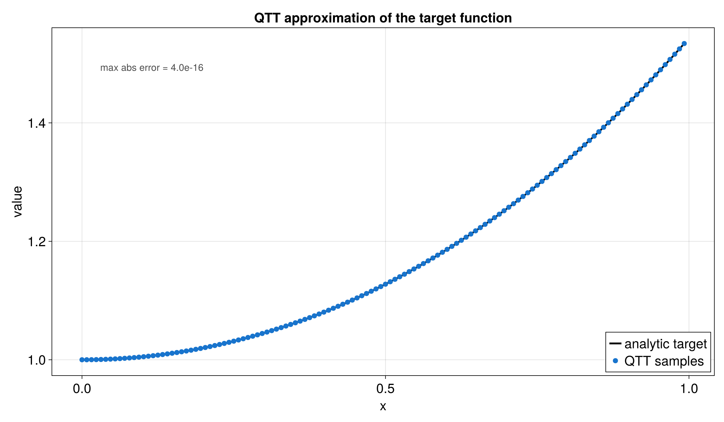
The points from the QTT lie on top of the direct function values. The next plot shows the bond dimensions along the QTT chain. In examples with a visible peak, that peak would mean that part of the grid needs more internal information than its neighbors.