Interpolative QTT

Interpolative QTT builds a tensor train by sampling a function through local Chebyshev-Lobatto interpolation. This is useful when the function is already given on a physical interval and known nonsmooth or sharply localized points should stay on a multiscale refinement path.

Runnable source: docs/tutorial-code/src/bin/interpolative_qtt.rs

Key API Pieces

Use interpolate_single_scale for a smooth one-dimensional function on one interval. The result is a binary TensorTrain, so the site index [0, 0, ...] evaluates the left endpoint of the sampled interval.

fn main() -> anyhow::Result<()> {
use tensor4all_interpolativeqtt::{
    interpolate_single_scale, AbstractTensorTrain, InterpolativeQttOptions,
};

let options = InterpolativeQttOptions::default().with_tolerance(1e-12);
let tt = interpolate_single_scale(
    |x| (-x * x).exp(),
    -1.0,
    1.0,
    5,
    12,
    &options,
)?;

let value = tt.evaluate(&[0, 0, 0, 0, 0])?;
assert!((value - (-1.0_f64).exp()).abs() < 1e-10);
Ok(())
}

Use interpolate_multi_scale when a known location should remain refined. The following target is a finite, softened version of 1 / r^2; the point x = 0 is still the sharp feature.

fn main() -> anyhow::Result<()> {
use tensor4all_interpolativeqtt::{
    interpolate_multi_scale, AbstractTensorTrain, InterpolativeQttOptions,
};

let epsilon = 0.2_f64;
let inverse_square = |x: f64| 1.0 / (x.abs() + epsilon).powi(2);
let options = InterpolativeQttOptions::default().with_tolerance(1e-12);
let tt = interpolate_multi_scale(
    inverse_square,
    -1.0,
    1.0,
    5,
    16,
    &[0.0],
    &options,
)?;

let value = tt.evaluate(&[0, 0, 0, 0, 0])?;
assert!((value - inverse_square(-1.0)).abs() < 1e-8);
Ok(())
}

The multidimensional constructor fuses all variables at the same bit level. For two variables each site has dimension 4, corresponding to the two binary digits at that level.

fn main() -> anyhow::Result<()> {
use tensor4all_interpolativeqtt::{
    interpolate_multi_scale_nd, AbstractTensorTrain, InterpolativeQttOptions,
};

let epsilon = 0.2_f64;
let radial_inverse_square = |x: &[f64]| {
    1.0 / (x[0] * x[0] + x[1] * x[1] + epsilon * epsilon)
};
let options = InterpolativeQttOptions::default().with_tolerance(1e-12);
let tt = interpolate_multi_scale_nd(
    radial_inverse_square,
    &[-1.0, -1.0],
    &[1.0, 1.0],
    4,
    8,
    &[vec![0.0, 0.0]],
    &options,
)?;

assert_eq!(tt.site_dims(), vec![4, 4, 4, 4]);
let value = tt.evaluate(&[0, 0, 0, 0])?;
assert!((value - radial_inverse_square(&[-1.0, -1.0])).abs() < 1e-8);
Ok(())
}

The tutorial binary runs these three constructions and writes CSV output for the plots below.

What It Computes

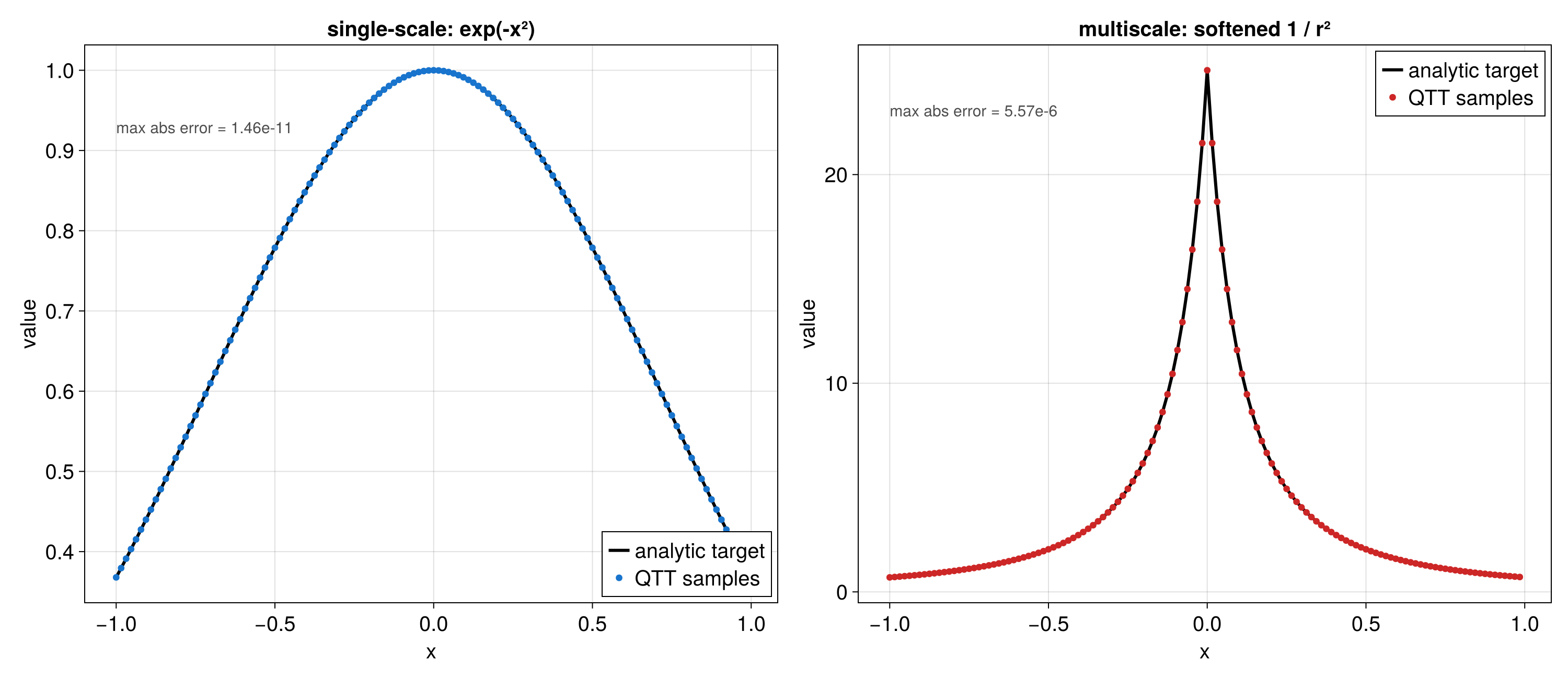
The first example uses single-scale interpolation for exp(-x^2). The second uses multiscale interpolation for a softened one-dimensional inverse-square profile, keeping the origin on the refinement path.

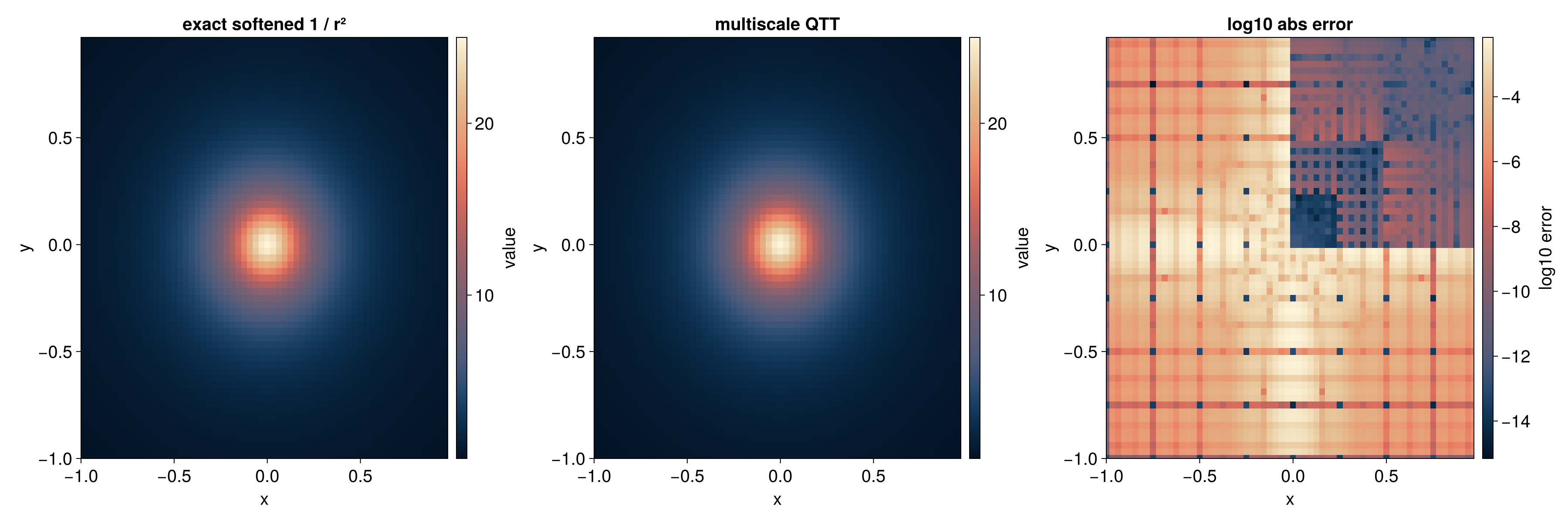
The third example uses interpolate_multi_scale_nd for a two-dimensional softened radial inverse-square profile. The error plot uses log10 absolute error so both the peak and the background remain visible.

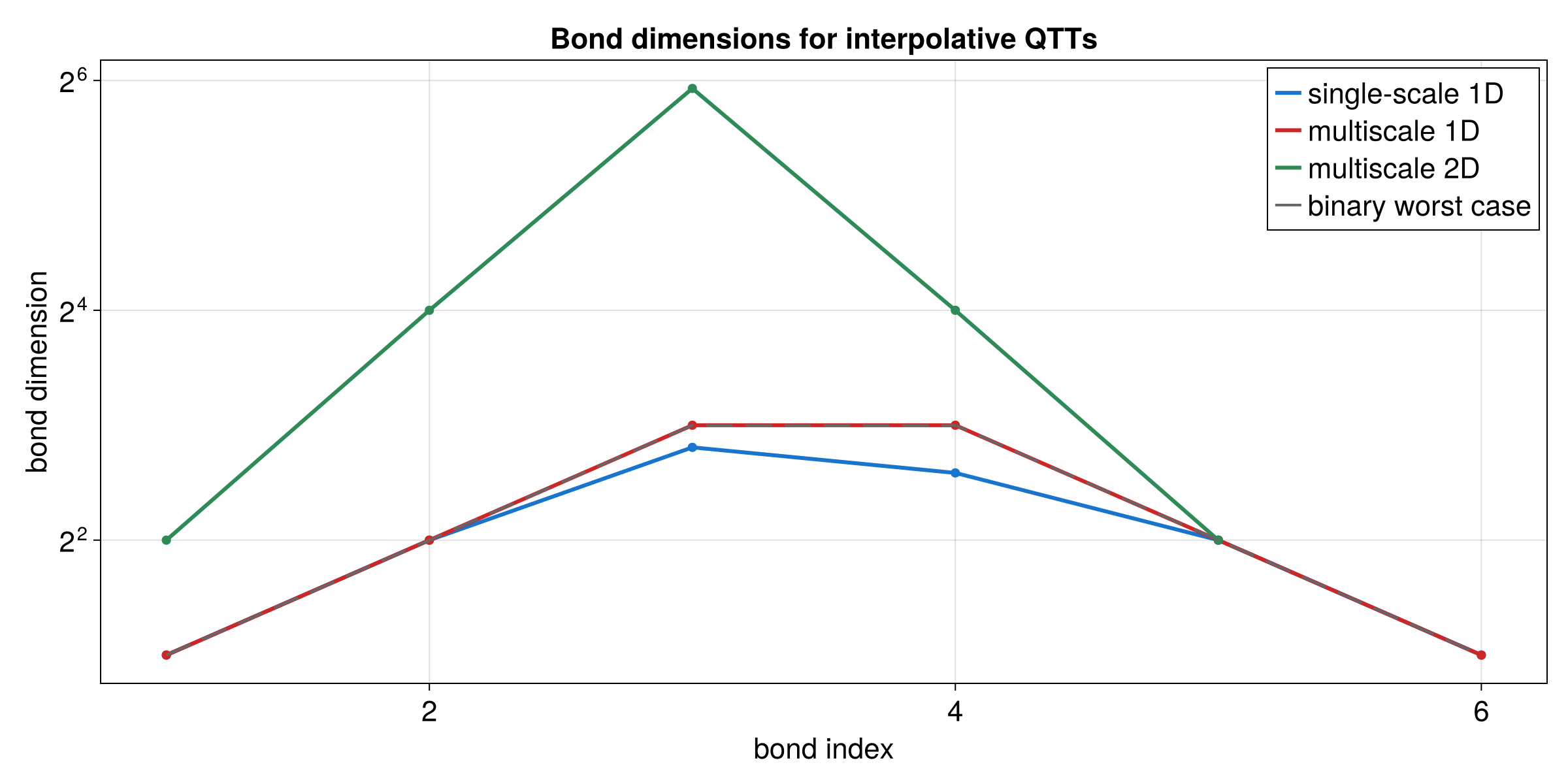
The final plot compares the bond dimensions for all three examples. The multiscale cases need larger internal spaces near the refined point, and the two-dimensional fused sites are more expensive than the one-dimensional sites.