Click here to download the notebook locally.

Quantum Fourier Transform

using LaTeXStrings
using Plots

import QuanticsGrids as QG
import TensorCrossInterpolation as TCI
using QuanticsTCI: quanticscrossinterpolate, quanticsfouriermpo

1D Fourier transform

\[ %\newcommand{\hf}{\hat{f}} %Fourier transform of \bff %\newcommand{\hF}{\hat{F}} \]

Consider a discrete function \(f_m \in \mathbb{C}^M\), e.g. the discretization, \(f_m = f(x(m))\), of a one-dimensional function \(f(x)\) on a grid \(x(m)\). Its discrete Fourier transform (DFT) is

\[ \hat{f}_k = \sum_{m=0}^{M-1} T_{km} f_m , \qquad T_{km} = \tfrac{1}{\sqrt{M}} e^{- i 2 \pi k \cdot m /M} . \]

For a quantics grid, \(M = 2^\mathcal{R}\) is exponentially large and the (naive) DFT exponentially expensive to evaluate. However, the QTT representation of \(T\) is known to have a low-rank structure and can be represented as a tensor train with small bond dimensions.

Thus, if the input function \(f\) is given in the quantics representation as

,

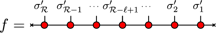\(\hat{f} = T f\) can be computed by efficiently contracting the tensor trains for \(T\) and \(f\) and recompressing the result:

.

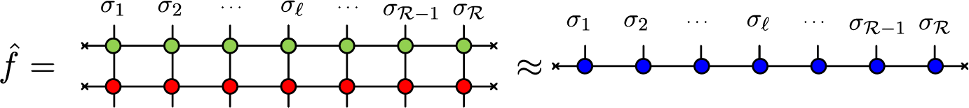Note that after the Fourier transform, the quantics indices \(\sigma_1,\cdots,\sigma_\mathcal{R}\) are ordered in the inverse order of the input indices \(\sigma'_1,\cdots,\sigma'_\mathcal{R}\). This allows construction of the DFT operator with small bond dimensions.

We consider a function \(f(x)\), which is the sum of exponential functions, defined on interval \([0,1]\):

\[ f(x) = \sum_p \frac{c_p}{1 - e^{-\epsilon_p}} e^{-\epsilon_p x}. \]

Its Fourier transform is given by

\[ \hat{f}_k = \int_0^1 dx \, f(x) e^{i \omega_k x} = - \sum_p \frac{c_p}{i\omega_k - \epsilon_p}. \]

for \(k = 0, 1, \cdots \) and \(\omega_k = 2\pi k\).

If you are familiar with quantum field theory, you can think of \(f(x)\) as a bosonic correlation function.

coeffs = [1.0, 1.0]
ϵs = [100.0, -50.0]

_exp(x, ϵ) = exp(-ϵ * x)/ (1 - exp(-ϵ))

fx(x) = sum(coeffs .* _exp.(x, ϵs))

fx (generic function with 1 method)

plotx = range(0, 1; length=1000)

plot(plotx, fx.(plotx))
xlabel!(L"x")
ylabel!(L"f(x)")

First, we construct a QTT representation of the function \(f(x)\).

R = 40
xgrid = QG.DiscretizedGrid{1}(R, 0, 1)

qtci, ranks, errors = quanticscrossinterpolate(Float64, fx, xgrid; tolerance=1e-10)

(QuanticsTCI.QuanticsTensorCI2{Float64}(TensorCrossInterpolation.TensorCI2{Float64} with rank 2, QuanticsGrids.DiscretizedGrid{1}(40, (0.0,), (1.0,), 2, :fused, false), TensorCrossInterpolation.CachedFunction{Float64, UInt128} with 2066 entries), [2, 2, 2], [2.793464338512118e-16, 2.220446049250313e-16, 2.220446049250313e-16])

Second, we compute the Fourier transform of \(f(x)\) using the QTT representation of \(f(x)\) and the QTT representation of the DFT operator \(T\):

\[ \hat{f}_k = \int_0^1 dx \, f(x) e^{i \omega_k x} \approx \frac{1}{M} \sum_{m=0}^{M-1} f_m e^{i 2 \pi k m / M} = \frac{1}{\sqrt{M}} \sum_{m=0}^{M-1} T_{km} f_m. \]

for \(k = 0, \ldots, M-1\) and \(\omega_k = 2\pi k\). This can be implemented as follows.

# Construct QTT representation of T_{km}
fouriertt = quanticsfouriermpo(R; sign=1.0, normalize=true)

# Apply T_{km} to the QTT representation of f(x)
sitedims = [[2,1] for _ in 1:R]
ftt = TCI.TensorTrain(qtci.tci)
hftt = TCI.contract(fouriertt, ftt; algorithm=:naive, tolerance=1e-8)

hftt *= 1/sqrt(2)^R

@show hftt
;

hftt = TensorCrossInterpolation.TensorTrain{ComplexF64, 3} of rank 18

Let us compare the result with the exact Fourier transform of \(f(x)\).

kgrid = QG.InherentDiscreteGrid{1}(R, 0) # 0, 1, ..., 2^R-1

_expk(k, ϵ) = -1 / (2π * k * im - ϵ)
hfk(k) = sum(coeffs .* _expk.(k, ϵs)) # k = 0, 1, 2, ..., 2^R-1

plotk = collect(0:300)
y = [hftt(reverse(QG.origcoord_to_quantics(kgrid, x))) for x in plotk] # Note: revert the order of the quantics indices
p1 = plot()
plot!(p1, plotk, real.(y), marker=:+, label="QFT")
plot!(p1, plotk, real.(hfk.(plotk)), marker=:x, label="Reference")
xlabel!(p1, L"k")
ylabel!(p1, L"\mathrm{Re}~\hat{f}(k)")

p2 = plot()
plot!(p2, plotk, imag.(y), marker=:+, label="QFT")
plot!(p2, plotk, imag.(hfk.(plotk)), marker=:x, label="Reference")
xlabel!(L"k")
ylabel!(L"\mathrm{Im}~\hat{f}(k)")

plot(p1, p2, size=(800, 500))

The exponentially large quantics grid allows to compute the Fourier transform with high accuracy at high frequencies. To check this, let us compare the results at high frequencies.

plotk = [10^n for n in 1:5]
@assert maximum(plotk) <= 2^R-1
y = [hftt(reverse(QG.origcoord_to_quantics(kgrid, x))) for x in plotk] # Note: revert the order of the quantics indices

p1 = plot()

plot!(p1, plotk, abs.(real.(y)), marker=:+, label="QFT", xscale=:log10, yscale=:log10)
plot!(p1, plotk, abs.(real.(hfk.(plotk))), marker=:x, label="Reference", xscale=:log10, yscale=:log10)
xlabel!(p1, L"k")
ylabel!(p1, L"\mathrm{Re}~\hat{f}(k)")

p2 = plot()

plot!(p2, plotk, abs.(imag.(y)), marker=:+, label="QFT", xscale=:log10, yscale=:log10)
plot!(p2, plotk, abs.(imag.(hfk.(plotk))), marker=:x, label="Reference", xscale=:log10, yscale=:log10)
xlabel!(p2, L"k")
ylabel!(p2, L"\mathrm{Im}~\hat{f}(k)")

plot(p1, p2, size=(800, 500))

You may use ITensors.jl to compute the Fourier transform of the function \(f(x)\). The following code explains how to do this.

import TCIITensorConversion
using ITensors
import Quantics: fouriertransform, Quantics

sites_m = [Index(2, "Qubit,m=$m") for m in 1:R]
sites_k = [Index(2, "Qubit,k=$k") for k in 1:R]

fmps = MPS(ftt; sites=sites_m)

# Apply T_{km} to the MPS representation of f(x) and reply the result by 1/sqrt(M)
# tag="m" is used to indicate that the MPS is in the "m" basis.
hfmps = (1/sqrt(2)^R) * fouriertransform(fmps; sign=1, tag="m", sitesdst=sites_k)

[ Info: Precompiling Quantics [87f76fb3-a40a-40c9-a63c-29fcfe7b7547]

MPS
[1] ((dim=2|id=157|"l=1,link"), (dim=2|id=440|"Qubit,k=40"))
[2] ((dim=2|id=233|"Qubit,k=39"), (dim=4|id=397|"l=2,link"), (dim=2|id=157|"l=1,link"))
[3] ((dim=2|id=426|"Qubit,k=38"), (dim=7|id=135|"l=3,link"), (dim=4|id=397|"l=2,link"))
[4] ((dim=2|id=210|"Qubit,k=37"), (dim=7|id=365|"l=4,link"), (dim=7|id=135|"l=3,link"))
[5] ((dim=2|id=923|"Qubit,k=36"), (dim=7|id=844|"l=5,link"), (dim=7|id=365|"l=4,link"))
[6] ((dim=2|id=197|"Qubit,k=35"), (dim=8|id=124|"l=6,link"), (dim=7|id=844|"l=5,link"))
[7] ((dim=2|id=318|"Qubit,k=34"), (dim=8|id=987|"l=7,link"), (dim=8|id=124|"l=6,link"))
[8] ((dim=2|id=696|"Qubit,k=33"), (dim=8|id=455|"l=8,link"), (dim=8|id=987|"l=7,link"))
[9] ((dim=2|id=33|"Qubit,k=32"), (dim=8|id=13|"l=9,link"), (dim=8|id=455|"l=8,link"))
[10] ((dim=2|id=220|"Qubit,k=31"), (dim=8|id=312|"l=10,link"), (dim=8|id=13|"l=9,link"))
[11] ((dim=2|id=904|"Qubit,k=30"), (dim=7|id=432|"l=11,link"), (dim=8|id=312|"l=10,link"))
[12] ((dim=2|id=817|"Qubit,k=29"), (dim=7|id=713|"l=12,link"), (dim=7|id=432|"l=11,link"))
[13] ((dim=2|id=168|"Qubit,k=28"), (dim=7|id=84|"l=13,link"), (dim=7|id=713|"l=12,link"))
[14] ((dim=2|id=562|"Qubit,k=27"), (dim=7|id=531|"l=14,link"), (dim=7|id=84|"l=13,link"))
[15] ((dim=2|id=206|"Qubit,k=26"), (dim=7|id=572|"l=15,link"), (dim=7|id=531|"l=14,link"))
[16] ((dim=2|id=12|"Qubit,k=25"), (dim=7|id=690|"l=16,link"), (dim=7|id=572|"l=15,link"))
[17] ((dim=2|id=428|"Qubit,k=24"), (dim=7|id=917|"l=17,link"), (dim=7|id=690|"l=16,link"))
[18] ((dim=2|id=76|"Qubit,k=23"), (dim=7|id=825|"l=18,link"), (dim=7|id=917|"l=17,link"))
[19] ((dim=2|id=58|"Qubit,k=22"), (dim=7|id=38|"l=19,link"), (dim=7|id=825|"l=18,link"))
[20] ((dim=2|id=571|"Qubit,k=21"), (dim=6|id=5|"l=20,link"), (dim=7|id=38|"l=19,link"))
[21] ((dim=2|id=188|"Qubit,k=20"), (dim=6|id=641|"l=21,link"), (dim=6|id=5|"l=20,link"))
[22] ((dim=2|id=214|"Qubit,k=19"), (dim=6|id=293|"l=22,link"), (dim=6|id=641|"l=21,link"))
[23] ((dim=2|id=611|"Qubit,k=18"), (dim=6|id=169|"l=23,link"), (dim=6|id=293|"l=22,link"))
[24] ((dim=2|id=189|"Qubit,k=17"), (dim=6|id=709|"l=24,link"), (dim=6|id=169|"l=23,link"))
[25] ((dim=2|id=793|"Qubit,k=16"), (dim=6|id=746|"l=25,link"), (dim=6|id=709|"l=24,link"))
[26] ((dim=2|id=616|"Qubit,k=15"), (dim=6|id=97|"l=26,link"), (dim=6|id=746|"l=25,link"))
[27] ((dim=2|id=24|"Qubit,k=14"), (dim=6|id=588|"l=27,link"), (dim=6|id=97|"l=26,link"))
[28] ((dim=2|id=316|"Qubit,k=13"), (dim=5|id=725|"l=28,link"), (dim=6|id=588|"l=27,link"))
[29] ((dim=2|id=379|"Qubit,k=12"), (dim=5|id=894|"l=29,link"), (dim=5|id=725|"l=28,link"))
[30] ((dim=2|id=408|"Qubit,k=11"), (dim=5|id=533|"l=30,link"), (dim=5|id=894|"l=29,link"))
[31] ((dim=2|id=202|"Qubit,k=10"), (dim=5|id=388|"l=31,link"), (dim=5|id=533|"l=30,link"))
[32] ((dim=2|id=913|"Qubit,k=9"), (dim=5|id=24|"l=32,link"), (dim=5|id=388|"l=31,link"))
[33] ((dim=2|id=746|"Qubit,k=8"), (dim=5|id=710|"l=33,link"), (dim=5|id=24|"l=32,link"))
[34] ((dim=2|id=990|"Qubit,k=7"), (dim=5|id=875|"l=34,link"), (dim=5|id=710|"l=33,link"))
[35] ((dim=2|id=402|"Qubit,k=6"), (dim=4|id=771|"l=35,link"), (dim=5|id=875|"l=34,link"))
[36] ((dim=2|id=71|"Qubit,k=5"), (dim=4|id=532|"l=36,link"), (dim=4|id=771|"l=35,link"))
[37] ((dim=2|id=508|"Qubit,k=4"), (dim=4|id=745|"l=37,link"), (dim=4|id=532|"l=36,link"))
[38] ((dim=2|id=287|"Qubit,k=3"), (dim=4|id=339|"l=38,link"), (dim=4|id=745|"l=37,link"))
[39] ((dim=2|id=5|"Qubit,k=2"), (dim=2|id=560|"l=39,link"), (dim=4|id=339|"l=38,link"))
[40] ((dim=2|id=985|"Qubit,k=1"), (dim=2|id=560|"l=39,link"))

# Evaluate Ψ for a given index
_evaluate(Ψ::MPS, sites, index::Vector{Int}) = only(reduce(*, Ψ[n] * onehot(sites[n] => index[n]) for n in 1:length(Ψ)))

_evaluate (generic function with 1 method)

@assert maximum(plotk) <= 2^R-1
y = [_evaluate(hfmps, reverse(sites_k), reverse(QG.origcoord_to_quantics(kgrid, x))) for x in plotk] # Note: revert the order of the quantics indices

p1 = plot()
plot!(p1, plotk, abs.(real.(y)), marker=:+, label="QFT")
plot!(p1, plotk, abs.(real.(hfk.(plotk))), marker=:x, label="Reference")
xlabel!(p1, L"k")
ylabel!(p1, L"\mathrm{Re}~\hat{f}(k)")

p2 = plot()
plot!(p2, plotk, abs.(imag.(y)), marker=:+, label="QFT")
plot!(p2, plotk, abs.(imag.(hfk.(plotk))), marker=:x, label="Reference")
xlabel!(p2, L"k")
ylabel!(p2, L"\mathrm{Im}~\hat{f}(k)")

plot(p1, p2, size=(800, 500))

2D Fourier transform

We now consider a two-dimensional function \(f(x, y) = \frac{1}{(1 - e^{-\epsilon})(1 - e^{-\epsilon'})} e^{-\epsilon x - \epsilon' y}\) defined on the interval \([0,1]^2\).

Its Fourier transform is given by

\[ \hat{f}_{kl} = \int_0^1 \int_0^1 dx dy \, f(x, y) e^{i \omega_k x + i\omega_l y} \approx \frac{1}{M^2} \sum_{m,n=0}^{M-1} f_{mn} e^{i 2 \pi (k m + l n) / M} = \frac{1}{M} \sum_{m,n=0}^{M-1} T_{km} T_{ln} f_{mn}. \]

The exact form of the Fourier transform is

\[ \hat{f}_{kl} = \frac{1}{(i\omega_k - \epsilon) (i\omega_l - \epsilon')}. \]

for \(k, l = 0, 1, \cdots \), \(\omega_k = 2\pi k\) and \(\omega_l = 2\pi l\).

The 2D Fourier transform can be numerically computed in QTT format (with interleaved representation) in a straightforward way using Quantics.jl.

ϵ = 1.0
ϵprime = 2.0
fxy(x, y) = _exp(x, ϵ) * _exp(y, ϵprime)

# 2D quantics grid using interleaved unfolding scheme
xygrid = QG.DiscretizedGrid{2}(R, (0, 0), (1, 1); unfoldingscheme=:interleaved)

# Resultant QTT representation of f(x, y) has bond dimension of 1.
qtci_xy, ranks_xy, errors_xy = quanticscrossinterpolate(Float64, fxy, xygrid; tolerance=1e-10)

(QuanticsTCI.QuanticsTensorCI2{Float64}(TensorCrossInterpolation.TensorCI2{Float64} with rank 1, QuanticsGrids.DiscretizedGrid{2}(40, (0.0, 0.0), (1.0, 1.0), 2, :interleaved, false), TensorCrossInterpolation.CachedFunction{Float64, UInt128} with 4918 entries), [1, 1, 1], [1.213634401775041e-16, 1.213634401775041e-16, 1.213634401775041e-16])

# for discretizing `y`
sites_n = [Index(2, "Qubit,n=$n") for n in 1:R]

sites_l = [Index(2, "Qubit,l=$l") for l in 1:R]

sites_mn = collect(Iterators.flatten(zip(sites_m, sites_n)))

fmps2 = MPS(TCI.TensorTrain(qtci_xy.tci); sites=sites_mn)
siteinds(fmps2)

80-element Vector{Index{Int64}}:
 (dim=2|id=479|"Qubit,m=1")
 (dim=2|id=591|"Qubit,n=1")
 (dim=2|id=60|"Qubit,m=2")
 (dim=2|id=108|"Qubit,n=2")
 (dim=2|id=497|"Qubit,m=3")
 (dim=2|id=592|"Qubit,n=3")
 (dim=2|id=331|"Qubit,m=4")
 (dim=2|id=369|"Qubit,n=4")
 (dim=2|id=10|"Qubit,m=5")
 (dim=2|id=75|"Qubit,n=5")
 (dim=2|id=117|"Qubit,m=6")
 (dim=2|id=971|"Qubit,n=6")
 (dim=2|id=417|"Qubit,m=7")
 ⋮
 (dim=2|id=385|"Qubit,m=35")
 (dim=2|id=368|"Qubit,n=35")
 (dim=2|id=245|"Qubit,m=36")
 (dim=2|id=89|"Qubit,n=36")
 (dim=2|id=428|"Qubit,m=37")
 (dim=2|id=950|"Qubit,n=37")
 (dim=2|id=916|"Qubit,m=38")
 (dim=2|id=401|"Qubit,n=38")
 (dim=2|id=651|"Qubit,m=39")
 (dim=2|id=302|"Qubit,n=39")
 (dim=2|id=286|"Qubit,m=40")
 (dim=2|id=41|"Qubit,n=40")

# Fourier transform for x
tmp_ = (1/sqrt(2)^R) * fouriertransform(fmps2; sign=1, tag="m", sitesdst=sites_k, cutoff=1e-20)

# Fourier transform for y
hfmps2 = (1/sqrt(2)^R) * fouriertransform(tmp_; sign=1, tag="n", sitesdst=sites_l, cutoff=1e-20)

siteinds(hfmps2)

80-element Vector{Index{Int64}}:
 (dim=2|id=440|"Qubit,k=40")
 (dim=2|id=723|"Qubit,l=40")
 (dim=2|id=233|"Qubit,k=39")
 (dim=2|id=163|"Qubit,l=39")
 (dim=2|id=426|"Qubit,k=38")
 (dim=2|id=860|"Qubit,l=38")
 (dim=2|id=210|"Qubit,k=37")
 (dim=2|id=240|"Qubit,l=37")
 (dim=2|id=923|"Qubit,k=36")
 (dim=2|id=221|"Qubit,l=36")
 (dim=2|id=197|"Qubit,k=35")
 (dim=2|id=598|"Qubit,l=35")
 (dim=2|id=318|"Qubit,k=34")
 ⋮
 (dim=2|id=402|"Qubit,k=6")
 (dim=2|id=485|"Qubit,l=6")
 (dim=2|id=71|"Qubit,k=5")
 (dim=2|id=399|"Qubit,l=5")
 (dim=2|id=508|"Qubit,k=4")
 (dim=2|id=926|"Qubit,l=4")
 (dim=2|id=287|"Qubit,k=3")
 (dim=2|id=247|"Qubit,l=3")
 (dim=2|id=5|"Qubit,k=2")
 (dim=2|id=612|"Qubit,l=2")
 (dim=2|id=985|"Qubit,k=1")
 (dim=2|id=591|"Qubit,l=1")

For convinience, we swap the order of the indices.

# Convert to fused representation and swap the order of the indices
hfmps2_fused = MPS(reverse([hfmps2[2*n-1] * hfmps2[2*n] for n in 1:R]))

# From fused to interleaved representation
sites_kl = collect(Iterators.flatten(zip(sites_k, sites_l)))
hfmps2_reverse = Quantics.rearrange_siteinds(hfmps2_fused, [[x] for x in sites_kl])
siteinds(hfmps2_reverse)

80-element Vector{Index{Int64}}:
 (dim=2|id=985|"Qubit,k=1")
 (dim=2|id=591|"Qubit,l=1")
 (dim=2|id=5|"Qubit,k=2")
 (dim=2|id=612|"Qubit,l=2")
 (dim=2|id=287|"Qubit,k=3")
 (dim=2|id=247|"Qubit,l=3")
 (dim=2|id=508|"Qubit,k=4")
 (dim=2|id=926|"Qubit,l=4")
 (dim=2|id=71|"Qubit,k=5")
 (dim=2|id=399|"Qubit,l=5")
 (dim=2|id=402|"Qubit,k=6")
 (dim=2|id=485|"Qubit,l=6")
 (dim=2|id=990|"Qubit,k=7")
 ⋮
 (dim=2|id=197|"Qubit,k=35")
 (dim=2|id=598|"Qubit,l=35")
 (dim=2|id=923|"Qubit,k=36")
 (dim=2|id=221|"Qubit,l=36")
 (dim=2|id=210|"Qubit,k=37")
 (dim=2|id=240|"Qubit,l=37")
 (dim=2|id=426|"Qubit,k=38")
 (dim=2|id=860|"Qubit,l=38")
 (dim=2|id=233|"Qubit,k=39")
 (dim=2|id=163|"Qubit,l=39")
 (dim=2|id=440|"Qubit,k=40")
 (dim=2|id=723|"Qubit,l=40")

klgrid = QG.InherentDiscreteGrid{2}(R, (0, 0); unfoldingscheme=:interleaved)

sparse1dgrid = collect(0:4)

reconstdata = [
    _evaluate(hfmps2_reverse, sites_kl, QG.origcoord_to_quantics(klgrid, (k, l)))
    for k in sparse1dgrid, l in sparse1dgrid]

hfkl(k::Integer, l::Integer) = _expk(k, ϵ) * _expk(l, ϵprime)

exactdata = [hfkl(k, l) for k in sparse1dgrid, l in sparse1dgrid]

c1 = heatmap(real.(exactdata))
xlabel!(L"k")
ylabel!(L"l")
title!("Real part of Exact data")

c2 = heatmap(real.(reconstdata))
xlabel!(L"k")
ylabel!(L"l")
title!("Real part of Reconstructed data")

c3 = heatmap(abs.(exactdata .- reconstdata))
xlabel!(L"k")
ylabel!(L"l")
title!("Error")

plot(c1, c2, c3, size=(1500, 400), layout=(1, 3))